FlatPPL, the Flat Portable Probabilistic Language
FlatPPL is a declarative, inference-agnostic probabilistic language designed for authoring, sharing, and converting statistical models across scientific domains. It is intended both as a directly writable source language and as a portable representation that higher-level modeling frontends may emit. FlatPPL describes models as static directed acyclic graphs (DAGs) of named mathematical objects — variates, measures, functions, and likelihoods — in a single flat module-level namespace with no block structure, no loops, and no dynamic branching. Its canonical surface form is small and easy to parse. In addition to deterministic and stochastic nodes, the language provides a measure algebra for measures and Markov kernels. Measures, kernels, and deterministic functions can be reified from sub-DAGs with optional boundary inputs, making it possible to extract conditional kernels and deterministic functions from larger models without auxiliary variables. FlatPPL code can be stored in standalone files or embedded in languages like Python and Julia. FlatPPL defines profiles, subsets of the language that map to other probabilistic languages and standards. FlatPPL is accompanied by the Flat Probabilistic Intermediate Representation (FlatPIR), to facilitate term-rewriting for optimization and conversion between profiles.
Table of Contents
1 Context and motivation #
1.1 Goals and target audience #
Statistical modeling in the sciences requires tools that are both mathematically rigorous and practically durable. However, there is still a lack of common standards and infrastructure to express, share, combine and evaluate statistical models across modeling tools and languages. Models should be FAIR (Findable, Accessible, Interoperable, Reusable). We would like to evaluate the same models using different computational engines in multiple end-user languages — in physics, especially C++, Python, and Julia — on a wide variety of modern hardware platforms (including accelerator hardware).
This document proposes FlatPPL, a declarative statistical modeling language that aims to move us closer to these goals, both directly and in connection with existing statistical languages, standards and tools.
FlatPPL is inspired by modeling needs in physics. High Energy Physics (HEP) in particular has a decades-long tradition of rigorous statistical analysis, with code lifetimes measured in decades and a strong culture of reproducibility and model preservation. The particle physics community and related fields like astrophysics and nuclear physics are the primary initial target audience. FlatPPL itself, however, is carefully designed not to be physics-specific, but to be broadly usable for statistical scientific models in general.
New readers may want to read the first four sections (motivation, overview, value types, and language design), then consult the following reference-style chapters (measure algebra, functions, distributions) as needed. Later sections provide worked examples, interoperability guidance and more.
1.2 Probabilistic languages #
A probabilistic language is a formal language for declaring generative models — descriptions of how data could have been produced by a stochastic process (often called forward modeling). The literature partially distinguishes between probabilistic modeling languages and probabilistic programming languages, though the distinction is not always sharp. A probabilistic programming language is often understood to provide both model specification and automatic inference, though not all do. The term probabilistic modeling language is less common, but clearly expresses that inference is not part of the feature set.
FlatPPL is primarily declarative: it describes models, not inference procedures. The scientist writes a model that reads like a simulation recipe: start with a set of parameter values, compute derived quantities, and describe how observations arise from distributions that depend on those parameters. The source model is not an inference procedure or control-flow program. It denotes a static mathematical object that different algorithms can traverse or evaluate in different ways (see below).
FlatPPL does, however, also support likelihood object declarations and density evaluation. Density evaluation defines the semantics of likelihood objects and is also useful for density-based computations within deterministic parts of models. This goes beyond what most probabilistic modeling languages offer, which often have a purely Bayesian focus, but is important for a language that aims to mesh well with formats and frameworks like HS³ and RooFit, and to equally support both frequentist and Bayesian settings.
Algorithms can use a probabilistic model in two fundamental ways, commonly called generative mode and scoring mode:
- Generative mode (simulation): traverses the declared model graph forward and draws random values from probability distributions to produce synthetic data.
- Scoring mode (density evaluation): given parameters and observed values, calculate log-likelihood or log-posterior density values for frequentist and Bayesian inference methods.
In addition to density evaluation, FlatPPL also supports engine-deterministic random-value generation — making both generation and scoring first-class within the language. This enables test-data generation and scoring (likelihood and posterior density values) directly in FlatPPL, though in production these operations are typically driven externally via host-language engine APIs.
Together, generative and scoring mode form the basis for the full range of statistical workflows: maximum likelihood estimation, profile likelihood ratios, Bayesian posterior sampling, hypothesis testing, model comparison, goodness-of-fit checking, and simulation-based inference.
The key design requirements here are:
- Language-independent. Not tied to a specific programming language. The design must allow for implementation of generative and scoring mode in a wide variety of host languages.
- Inference-agnostic. Must serve both Bayesian and frequentist use cases.
- Not tied to a specific engine. No coupling to particular inference algorithms or computational backends.
- Long-lived. Code lifetimes in HEP have long been measured in decades and data preservation is becoming an increasing concern in many scientific fields. The design must be durable enough to outlast current software and hardware ecosystems.
- Expressive. Must allow us to express a wide corpus of models across many scientific domains.
Accelerator compatibility. Models that are expressed as a static DAG of bindings — with value shapes that are statically known or resolved at module-load time, no loops, no dynamic control flow, no shapes that change during evaluation, but with explicit support for elementwise operations — map naturally to accelerator-oriented IRs such as MLIR/StableHLO/XLA. Engines targeting high-performance backends (e.g., via JAX in Python or Reactant.jl in Julia) can lower operations on a model, like sampling or density/likelihood evaluation, to these IRs — without fundamental impedance mismatches for the large class of common models with static topology and statically known shapes.
1.3 A starting point: RooFit and HS³ #
The current principal building blocks for statistical modeling in High Energy Physics are RooFit (a C++ modeling toolkit in ROOT) and the HEP Statistics Serialization Standard (HS³), a JSON-based interchange format. pyhf is a JSON specification and Python implementation of the HistFactory template-fitting model class that originated in RooFit. While pyhf comes with a Python engine, both HS³ and pyhf JSON are model descriptions for which engines can be, and currently are being, implemented in multiple languages.
RooFit provides a rich and mature framework for building probability models. Its architecture is based on directed acyclic graphs (DAGs) that express computational dependencies between named objects.
As such, HS³ and pyhf successfully demonstrate how statistical semantics can be disentangled from a DSL that is tied to a specific host language like RooFit/HistFactory. HS³ is young, compared to RooFit, but already in use by the ATLAS collaboration for publishing likelihoods on HEPData.
However, RooFit and HistFactory were built for a specific scientific domain and lack features required in many other domains. HS³ (and pyhf) largely inherited these limitations:
- No distribution/PDF distinction. RooFit conflates distributions with their PDFs, and PDFs do not separate parameters from observables — the distinction arises from usage context (which variables appear in the dataset at fit time). This allows operations such as normalizing a likelihood function over parameter space and treating it as a probability density — an operation that is statistically ill-defined in general, since the likelihood is not a probability measure on parameter space.
- Only scalar variables. All variables are scalar workspace-global objects — there are no vector-valued parameters or variates. Record-like structures (e.g. named components of a multivariate normal) must be flattened into individually named scalars.
- No support for linear algebra.
- No support for complex numbers.
- Stochastic dependencies — one distribution’s variate is another’s parameter — require explicit conditional product construction. Stan-like stochastic graphs are foreign to the RooFit/HS³ approach.
The HS³ standard is written in a more cross-disciplinary fashion, with a clearer separation of some statistical concepts. In particular, it makes the forward-modeling approach that underpins RooFit more explicit. Some of the limitations above may be addressed in future versions of HS³, but others are fundamental, in particular the inability to express stochastic graphs.
The JSON format of HS³ (and pyhf) makes for easy machine-readability, but is not conducive to human readability and human authoring, especially for larger models. Models are often built in RooFit or more specialized tools and then exported to HS³. As RooFit is a fairly narrow C++-embedded DSL that directly expresses computational graphs, exporting to HS³ (built to match RooFit) is straightforward.
This leaves us with an authoring problem: statistical DSLs that are more expressive or allow for broad use of host-language concepts are much harder to map to a language-independent representation, and even harder to map to one not specifically matched to them. On the other hand, models expressed in a standard like HS³ are themselves highly portable, but how do we generate them in scientific domains where models are written in languages or created by tools that may use different semantic models?
1.4 Other probabilistic languages #
There is a rich landscape of stochastic/probabilistic languages; in addition to RooFit, HS³ and pyhf, the following are particularly relevant in our context:
Stan (Carpenter et al., 2017) is a very strong candidate for longevity: it has a large and active user and developer community, bindings for multiple languages (R, Python, Julia and others), and solid funding. However:
- Stan is fundamentally Bayesian, though modern Stan does
support some frequentist workflows. The language is designed
around the
modelblock, which defines a joint probability distribution over parameters and observations with no syntactic separation between prior and observation model. - Stan is a full probabilistic programming language with rich syntax, tightly coupled to a specific compiler and runtime (stanc → C++). There is no independent implementation, so it is not suited to be a language-independent interchange format.
Pyro/NumPyro, Turing.jl, PyMC are powerful Bayesian-centric systems. They couple a DSL embedded in their host languages (Python or Julia) with a set of inference algorithms that are specific to each. Independent implementations of the modeling DSLs are not feasible, however, as they leverage very large subsets of the host language and so are tied to that language.
GraphPPL.jl (used by RxInfer) separates model specification from inference backend, which is architecturally what we want. It is Julia-specific and Bayesian-focused and trades generality for high-speed inference.
Hakaru (Narayanan et al., 2016) has elegant semantics built on the Giry monad, expressing programs as measure expressions with support for both frequentist and Bayesian reasoning. Hakaru, however, is based on and tied to Haskell, and does not appear to be actively maintained.
This list should not be seen as exhaustive, nor as an attempt to compare, let alone rate or critique, these languages. Any misrepresentations are unintentional and the authors will be happy to correct them.
All of these languages are powerful and well-designed. FlatPPL is not meant to replace any of them, but to help bridge gaps between expressive power, portability, longevity and DSL-independent model authoring. While FlatPPL is suitable for direct model authoring (see below), different communities use different tools for good reasons. FlatPPL is not an attempt to establish a universal authoring standard for statistical models. Nor is it an attempt to establish a single universal model exchange standard.
1.5 Use cases for FlatPPL #
Model representation and evaluation. Models can be directly authored in or converted to FlatPPL and then evaluated via FlatPPL implementations/engines. FlatPPL is designed for efficient implementation in multiple host languages and use of accelerator hardware. Once stable, FlatPPL will aim for long-term backward-compatibility.
Model conversion. FlatPPL is designed to be a suitable intermediate stage when converting models between different stochastic languages and formats. Tracing compilers and other relevant technologies have become increasingly popular and powerful in recent years, so the technological basis seems largely in place. FlatPPL intentionally supports explicit distribution composition (like RooFit) as well as stochastic graphs (like Stan, Pyro and others) so it can connect across the spectrum of stochastic languages.
Design and reasoning. FlatPPL explores a set of mathematical and statistical semantics that is broad, coherent and rigorous, and has the potential to inform design or extension of other probabilistic languages and standards. FlatPPL also comes with a simple and readable canonical syntax that makes it suitable as a reasoning aid in cases where mathematical notation would still be too informal or too dependent on context. The semantics of FlatPPL are, however, independent of this canonical syntax.
2 Language overview #
2.1 FlatPPL in a nutshell #
The name FlatPPL reflects the language’s most distinctive design choices. Probabilistic models are expressed as static graphs of named mathematical objects — variates, measures, functions, and likelihoods — in a single flat module-level namespace, with no function blocks or block scopes, no loops and no dynamic branching. A FlatPPL document is a sequence of named bindings in static single-assignment (SSA) form. The order of statements is semantically irrelevant; the graph structure is determined by name references, not by textual position. Data is represented by ordinary values (arrays, records, tables).
This simplicity makes FlatPPL amenable to serialization, static analysis, and compilation to accelerator backends, while still being expressive enough to cover a wide range of models across scientific domains. The resulting graph structure is similar to an HS³ JSON document or a RooFit workspace, though FlatPPL concepts like random draws and measure/function reification do not currently exist in HS³ and RooFit. See the profiles and interoperability section on how FlatPPL maps to them.
Creating FlatPPL models. FlatPPL is intended both for direct authoring and as a target representation for models defined in other stochastic languages. Writing FlatPPL documents directly is practical for smaller and medium-sized models and for didactic settings. Users may prefer to use host-language frameworks to author models though, especially larger and complex models, or to use other DSLs to run, exchange and preserve models. FlatPPL is designed to be broad enough to make it a practical target from a wide variety of modeling frontends.
Converting FlatPPL models. FlatPPL defines profiles (see Profiles), specific subsets of the language for easy mapping to target probability languages and formats.
Canonical syntax. FlatPPL comes with a canonical surface form: a small, easy-to-parse syntax. See section Syntax for the grammar and host-language embedding options. This document uses the canonical syntax as a notation to define FlatPPL semantics and to present language examples. Note though that the semantics of FlatPPL are independent from this canonical syntax. The design of FlatPPL allows for alternative surface forms with the same semantics.
Canonical intermediate representation. FlatPPL also comes with a canonical intermediate representation (IR) based on S-expressions, the Flat Probabilistic Intermediate Representation (FlatPIR) (see Intermediate Representation). FlatPIR supports metadata like type and phase annotations and is suitable for automated term-rewriting, enabling code optimization and conversion between FlatPPL profiles. FlatPPL maps directly to and from FlatPIR, enabling round-tripping.
2.2 Implementation targets #
The scientific communities where we expect FlatPPL to see most use primarily work in C++/ROOT, Python, and Julia. Each ecosystem brings its own strengths and infrastructure for statistical modeling:
C++ / RooFit. RooFit is the most mature and widely deployed statistical modeling toolkit in high energy physics, but currently lacks some features required in other fields where it could play a role. FlatPPL is likely to target RooFit via HS³ conversion initially, though direct support is also possible. In either case the implementation strategy is evolution, not replacement: non-breaking additions to widen the semantic scope of RooFit and bring it as close to the scope of FlatPPL as feasible. See the HS³/RooFit profile section for details. Stan, as mentioned before, is very powerful but does not cover all of our requirements. Many strictly Bayesian FlatPPL models could be converted to Stan model blocks though and run on the Stan engine. Accelerator support for RooFit seems less likely for now in general.
Python. pyhf covers the HistFactory subset of HS³, zfit has partial support, and pyhs3 provides a first Python HS³ implementation. In regard to FlatPPL there is more room for direct support in the Python ecosystem than in C++/RooFit. JAX offers a natural path to accelerator-oriented execution via MLIR/StableHLO.
Julia. There is only a prototype HS³ implementation in Julia (HS3.jl). Julia has a rich ecosystem of statistics packages like Distributions.jl and MeasureBase.jl that provide an excellent basis for an inference-agnostic implementation of FlatPPL, orthogonal to inference packages like ProfileLikelihood.jl, BAT.jl and others. FlatPPL and HS³ models could be supported in Julia via the same graph engine. The Julia equivalent to JAX is Reactant.jl, like JAX it targets accelerators via MLIR/StableHLO.
2.3 A first example #
Before delving into the language more formally, here is a small example to convey the flavor of the FlatPPL language. This high energy physics model describes a simple particle mass measurement where the observed spectrum is a superposition of signal and background events, with a systematic uncertainty on the signal resolution:
%%%
# Particle mass measurement

Unbinned Poisson-process model: a Gaussian signal peak at known mass on a
falling exponential background, with a Gaussian-shifted resolution
systematic. Returns a likelihood object `L` parameterized by the expected
signal and background counts.
%%%
flatppl_compat = "0.3"

# Inputs: expected signal and background event counts
% Expected number of signal events.
n_sig = elementof(reals)
% Expected number of background events.
n_bkg = elementof(reals)

% Standard-normal systematic shift applied to the detector resolution.
raw_syst ~ Normal(mu = 0.0, sigma = 1.0)
resolution = 2.5 + 0.3 * raw_syst

# Signal: Gaussian peak at known mass, uncertain resolution
signal_shape = Normal(mu = 125.0, sigma = resolution)

# Background: falling exponential
background_shape = Exponential(rate = 0.05)

# Unbinned data
observed_data = [120.1, 124.8, 125.3, 130.2, 135.7, 142.0]

# Combined intensity: unnormalized superposition (weights = expected event counts)
intensity = superpose(
    weighted(n_sig, signal_shape),
    weighted(n_bkg, background_shape)
)

# Unbinned model: Poisson process over scalar mass values
events ~ PoissonProcess(intensity = intensity)

% Likelihood as a function of the expected event counts.
L = likelihoodof(kernelof(events), observed_data)
The example uses both kinds of textual annotation:
# for plain comments
(parser-discarded) and % / %%% for doc-comments.
Reading top to bottom, this is a generative recipe: declare
inputs, draw a systematic shift, compute the resolution, define
signal and background shapes, combine them as an unnormalized
superposition (where the weights encode expected event counts),
and draw events from the resulting Poisson process. Since the
event space is scalar (mass values), the
PoissonProcess produces an array variate, and the
observed data is a plain array of mass values. (This
top-to-bottom reading is for intuition only; semantically the
bindings form a dependency graph and may be resolved in any
topological order.) The same specification supports generative
mode (engines draw synthetic events) and scoring mode (engines
compute the log-likelihood at given parameter values).
Note. From a Bayesian perspective, the same
model can be read as having a prior
Normal(mu = 0.0, sigma = 1.0) on
raw_syst, with n_sig and
n_bkg as externally supplied hyperparameters or
model parameters. This illustrates FlatPPL’s inference-agnostic
design.
2.4 Core concepts #
FlatPPL has five kinds of first-class objects.
Abstract values denote real numbers,
integers, booleans, complex numbers, fixed-size arrays, and
records. They may be deterministic (literal constants, results
of ordinary functions, data, external inputs) or stochastic
(variates introduced by draw(...)). In generative
mode, each abstract value evaluates to a single concrete value;
for stochastic abstract values, that concrete value is generated
randomly once.
Kernels, measures and distributions.
Transition kernels are mappings from an input space to measures.
FlatPPL does not distinguish between a kernel with an empty
interface and a measure: in FlatPPL, such a kernel is a
measure (see variates and
measures). Normalized measures (kernels) are probability
measures (Markov kernels), also called probability
distributions. Variates can only be drawn from probability
measures. Otherwise, FlatPPL treats measures and kernels
uniformly in measure algebra (see measure algebra). Variates can
be reified as probability measures via lawof(...),
and as Markov kernels via kernelof(...) (see reification to measures and kernels and kernelof).
Likelihood objects represent the density of
a model evaluated at observed data, as a function of the model’s
input parameters. The observed data is bound to the likelihood
object when it is constructed. To prevent a mix-up of likelihood
and log-likelihood values, FlatPPL does not treat a likelihood
object as a function that returns the one or the other. Instead,
(log-)likelihood values are computed via
densityof(L, theta) and
logdensityof(L, theta) to make the choice explicit.
(See likelihoods and
posteriors for the full treatment.)
Functions compute result values from input
values in a deterministic fashion. See calling conventions and anonymous
functions for details. Values can be reified as functions
via functionof(...).
Tuples are ordered bundles of objects. Tuples may contain any objects except for other tuples (see Tuples).
Measures, likelihood objects, functions, and tuples are first-class in the sense that they can be bound to names, passed to operations and referenced by other bindings. However, they may not appear inside arrays, records, or tables.
Modules represent whole FlatPPL documents;
each FlatPPL source file is a module. A FlatPPL module can load
other modules (via load_module(module_filename))
and access objects in loaded modules via dot-syntax scoping
(loaded_module.some_object). Module objects give
access to another namespace, but are not themselves first-class
objects in the computational graph: they may not be passed to
functions or appear inside data structures. See multi-file models for details.
2.5 Language map #
The table below provides a compact overview of the language. Each family name links to the section where the constructs are documented. The lists are selected highlights, not exhaustive — see the linked sections for complete listings.
| Family | Constructs |
|---|---|
| Special operations | draw, lawof,
functionof, kernelof, fn,
fchain, bijection, fixed,
elementof, external,
valueset, vector,
checked |
| Interface adaptation | relabel |
| Measure combinators | weighted, logweighted,
normalize, totalmass,
superpose, joint,
jointchain, kchain,
markovchain, kscan, iid,
truncate, pushfwd,
locscale |
| Likelihoods and posteriors | likelihoodof, joint_likelihood,
densityof, logdensityof,
bayesupdate |
| Structural disintegration | disintegrate, restrict |
| Broadcasting | broadcast, broadcasted |
| Reductions and aggregation | reduce, scan,
aggregate, metricsum |
| Data access and reshaping | get, get0, cat,
record, tuple, all,
filter, selectbins,
reverse |
| Array and table generation | array, table,
rowstack, colstack,
partition, linspace,
extlinspace, fill, zeros,
ones, eye, onehot,
load_data |
| Binning | bincounts |
| Shape functions | polynomial, bernstein,
stepwise |
| Math and logic | identity, exp, log,
pow, sqrt, abs,
sin, cos, min,
max, floor, ceil,
round, div, mod,
gamma, loggamma, logit,
invlogit, probit,
invprobit, ifelse, land,
lor, lnot, lxor,
lany, lall |
| Predicates | isfinite, isinf,
isnan, iszero |
| Linear algebra | transpose, adjoint,
det, logabsdet, inv,
trace, linsolve,
lower_cholesky, cross |
| Operator functions | add, sub, mul,
divide, neg, equal,
unequal, lt, le,
gt, ge |
| Complex arithmetic | complex, real, imag,
conj, abs2, cis |
| Reductions | sum, mean, var,
prod, maximum, minimum,
lengthof |
| Norms and normalization | l1norm, l2norm,
linfnorm, l1unit, l2unit,
logsumexp, softmax,
logsoftmax |
| Distributions | Normal, Poisson,
PoissonProcess, BinnedPoissonProcess,
Exponential, Dirichlet, … |
| Fundamental measures | Lebesgue, Counting,
Dirac |
| Random value generation | rand, rngstate,
rnginit |
| Module operations | load_module, standard_module,
flatppl_compat |
| Constants | true, false, inf,
pi, im |
| Predefined sets | reals, posreals,
nonnegreals, unitinterval,
posintegers, nonnegintegers,
integers, booleans,
complexes, rngstates,
anything |
| Set constructors | interval, cartprod,
cartpow, stdsimplex |
| Selectors and operators | all (slicing), in
(membership) |
2.6 A tour of FlatPPL #
The following code blocks illustrate the main language features. Each construct is explained in detail in later sections. These snippets are independent and do not form a single model.
2.6.1 Values and collections #
Scalars, arrays, nested arrays, matrices, records, and basic operations:
# Scalars
x = 3.14
n = 42
b = true

# Collections
v = [1.0, 2.0, 3.0]
nested = [[1, 2], [3, 4]]
M = rowstack([[1, 2, 3], [4, 5, 6]])
r = record(mu=3.0, sigma=1.0)

# Indexing, field access, slicing
y = A[i]
z = A[i, j]
w = r.mu
col_j = M[:, j]

# Decomposition into named scalars
a, b, c ~ MvNormal(mu = mean, cov = cov_matrix)
p, q = some_record
l, m, n = some_tuple

# Arithmetic, comparisons, function calls
rate = efficiency * mu_sig + background
is_positive = x > 0
y = exp(x)
z = ifelse(is_positive, a, b)
combined = cat(record1, record2)
joined = cat(array1, array2)
2.6.2 Function calls #
Calling conventions:
Normal(mu = 0, sigma = 1)           # keyword
Normal(record(mu = 0, sigma = 1))   # record auto-splatting
exp(x)                              # positional
2.6.3 Complex arithmetic #
Constructing and calculating with complex values:
# Complex construction
z1 = complex(3.0, 2.0)
z2 = 3.0 + 2.0 * im               # equivalent
phase = cis(3 * pi / 4)           # unit-modulus complex from angle

# Complex arithmetic
A_total = A_sig * coupling + A_bkg

# Squared modulus (real-valued result)
intensity = abs2(A_total)

# Decomposition and conjugation
x = real(z1)
y = imag(z1)
z_bar = conj(z1)
2.6.4 Draws, measures, and the stochastic core #
draw, lawof,
functionof, and kernelof bridge
between values, measures, functions, and kernels:
# Inputs
mu = elementof(reals)
sigma = elementof(interval(0.0, inf))

# Random draw from a distribution
a ~ Normal(mu = mu, sigma = sigma)

# Extract the distribution governing a value
M = lawof(a)

b = 2 * a + 1

# Reify a deterministic sub-DAG as a function (boundary stops trace at `a`)
f = functionof(b, x = a)

# Stochastic sub-DAG reified as a kernel
K = kernelof(b, x = a)
2.6.5 Broadcasts #
broadcast applies functions or kernels
elementwise over arrays and tables:
# Function over array (keyword binding)
C = broadcast(f, x = A)

# Same, positional
C = broadcast(f, A)

# Kernel over array
D ~ broadcast(K, x = A)
2.6.6 Value-level operations #
Accessing and renaming values, and transforming measures based on that:
# Element and subset access
field_a = get(some_record, "a")
sub = get(some_record, ["a", "c"])

# Array to record conversion
named = relabel(some_array, ["a", "b", "c"])

# Structural relabeling of a measure
mvmodel = relabel(MvNormal(mu = some_mean, cov = some_cov), ["a", "b", "c"])

# Variable transformation
log_normal = pushfwd(x -> exp(x), Normal(mu = 0, sigma = 1))

# Projection (marginalizes out b)
marginal_ac = pushfwd(fn(get(_, ["a", "c"])), mvmodel)
2.6.7 Measure algebra and composition #
Combining, reweighting, and transforming measures some more:
# IID draws
xs ~ iid(Normal(mu = 0, sigma = 1), 100)

# Additive rate superposition
sp = superpose(weighted(n_sig, sig), bkg)

# Normalized mixture
mix = normalize(superpose(
    weighted(0.7, M1), weighted(0.3, M2)))

# Joint of independent components
j = joint(M1, M2)

# Marginalizing composition
pp = kchain(prior, forward_kernel)

# Hierarchical joint (retains both variates)
hj = jointchain(
    pushfwd(fn(relabel(_, ["a"])), M1),
    pushfwd(fn(relabel(_, ["b"])), K_b))

# Truncated (unnormalized) measure
positive_normal = truncate(Normal(mu = 0, sigma = 1),
    interval(0, inf))

# Fundamental measures and density-defined distributions
leb = Lebesgue(support = reals)
bern = fn(bernstein(coefficients = [c0, c1, c2], x = _))
smooth_shape = normalize(weighted(bern, Lebesgue(support = interval(lo, hi))))
2.6.8 Anonymous functions #
The fn(...) form wraps a hole expression — an
expression containing _ — to create an anonymous
function with positional parameters:
# Single hole — one-argument function
poly = fn(polynomial(coefficients = [a0, a1, a2], x = _))
squared = fn(_ ^ 2)

# Multi-hole: two-argument anonymous function
ratio_sq = fn((_ / _) ^ 2)
2.6.9 Interpolation, binning, and systematic variations #
Constructors for binned models and HistFactory-style yield arithmetic:
edges = linspace(0.0, 10.0, 5)
counts = bincounts(edges, event_data)

# Binned observation model via pushforward
binned_model = pushfwd(fn(bincounts(edges, _)),
    PoissonProcess(intensity = M_intensity))

# Interpolation for systematic variations (particle-physics standard module)
hepphys = standard_module("particle-physics", "0.1")
kappa = hepphys.interp_poly6_exp(0.95, 1.0, 1.05, alpha)
morphed = hepphys.interp_poly6_lin(tmpl_dn, nominal, tmpl_up, alpha)
2.6.10 Data #
Data is represented by ordinary values — no special data type:
observed_counts = [5, 12, 8, 3]
data_table = table(a = [1.1, 1.2], b = [2.1, 2.2])
2.6.11 Presets #
Advisory parameter/input values for use with a compatible function, kernel, or likelihood:
# Parameter starting values (advisory, not part of model semantics)
starting_values = record(mu_sig = 1.0, raw_syst = fixed(0.0), n_bkg = 50.0)
2.6.12 Analysis: likelihoods and posteriors #
Likelihood construction, combination, and posterior construction:
L = likelihoodof(kernelof(obs), data)
R = interval(2.0, 8.0)
L_sub = likelihoodof(normalize(truncate(kernelof(obs), R)), filter(fn(_ in R), data))
L_total = joint_likelihood(L1, L2)

# Unnormalized posterior
posterior = bayesupdate(L, prior)

# Deterministic function composition
pipeline = fchain(calc_kinematics, apply_cuts)
2.6.13 Modules and interface adaptation #
Module loading and parameter renaming:
# Load a module and optionally bind some of its inputs
sig = load_module("signal_channel.flatppl", mu = signal_strength, theta = nuisance)

sig_model = sig.model
L_sig = likelihoodof(sig.model, sig.data)
3 Value types and data model #
FlatPPL has a small, fixed set of value types. This section defines what kinds of values exist in the language, their invariants, and how they interact. Operations on values are documented in built-in functions.
3.1 Scalar types #
Real. Floating-point numbers like
3.14, -0.5, 1e-3.
Integer. Integer numbers like
42, 0, -7.
Bool. true or
false (lowercase). In arithmetic contexts,
false is promoted to zero and true to
one, permitting expressions such as true + true,
3 * false, and sum(mask) to count true
entries. Conditional and logical constructs
(ifelse, land, lor,
lnot, lxor) strictly require boolean
arguments; zero and one are not implicitly converted to
booleans.
Complex. A complex number. Constructed via
complex(re, im) or via arithmetic with the
imaginary unit im:
z1 = complex(3.0, 2.0)
z2 = 3.0 + 2.0 * im           # equivalent
phase = cis(3 * pi / 4)       # unit-modulus complex from angle
When a real and a complex value meet in arithmetic, the real is promoted to complex with zero imaginary part.
Scalar value categories and sets. FlatPPL
distinguishes boolean, integer, real, and complex scalar values
operationally. In particular, conditionals and logical operators
require boolean values. However, the predefined value sets
satisfy the canonical inclusions booleans integers reals, and there
is a canonical embedding of reals into
complexes. Arithmetic may use these canonical
embeddings implicitly where specified by the language.
3.2 Predefined constants #
| Name | Type | Description |
|---|---|---|
true, false |
Bool | Boolean constants |
inf |
Real | Positive infinity (). Used in
interval, extlinspace,
truncate |
pi |
Real | The mathematical constant |
im |
Complex | The imaginary unit (). Equivalent to
complex(0.0, 1.0) |
reals |
Set | The real numbers, with admitted (see note below).
Default support for Lebesgue |
posreals |
Set | The positive reals including : |
nonnegreals |
Set | The non-negative reals including : |
unitinterval |
Set | The unit interval |
posintegers |
Set | The positive integers |
nonnegintegers |
Set | The non-negative integers |
integers |
Set | The set of all integers (). Default support for
Counting |
booleans |
Set | The set |
complexes |
Set | The set of all complex numbers () |
rngstates |
Set | The set of RNG state values (algorithm-dependent opaque values) |
anything |
Set | Generic placeholder set for untyped interfaces (see sets) |
Note on infinities. posreals,
nonnegreals, and reals admit
inf (and, for reals,
-inf) as legal values. Strictly speaking, these are
subsets of the extended reals , not of . This is a deliberate
choice for compatibility with common numerical and statistical
libraries. When FlatPPL refers to
Lebesgue(support = reals), the reference measure is
the ordinary Lebesgue measure on the finite-real part; the
points carry zero
Lebesgue mass. Arithmetic on infinities follows IEEE 754
conventions.
The selector all and the hole token
_ are syntactic elements, not value constants; they
are documented in calling
conventions and anonymous functions.
3.3 Arrays #
Arrays are fixed-size, ordered, n-dimensional collections of scalar values (real, integer, boolean and complex values) or arrays.
Literal one-dimensional arrays are denoted as
[1.0, 2.0, 3.0] and may contain arbitrary valid
FlatPPL expressions that evaluate to allowed element types
(e.g. [a, b, 2 * c]).
One-dimensional arrays of scalars act as vectors for linear algebra (see built-in functions). In addition, transposed vectors are a distinct type in FlatPPL (see linear algebra). The term vector will represent both non-transposed vectors (one-dimensional arrays) and transposed vectors in the following, unless noted otherwise.
Vectors of vectors are not interpreted as matrices
implicitly, but can be turned into matrices explicitly using
rowstack or colstack (see array operations).
FlatPPL supports standard linear algebra operations (addition, multiplication) on scalars, vectors, and matrices.
3.4 Records #
Records comprise ordered named fields, written as
record(name1=val1, name2=val2, ...). Field values
may be scalars, arrays, or records. Field access uses dot
syntax: r.name1 (lowers to
get(r, "name1")); nested fields chain,
e.g. r.a.b. Field order is part of the record’s
identity: record(a=1, b=2) and
record(b=2, a=1) are distinct values. This is
significant for alignment with parameter spaces and for
deterministic serialization. Fields are accessed by name, not by
position — get(r, i) is not supported to avoid
ambiguity with row indexing on tables.
3.5 Presets #
Presets are global fixed records and sets that hint suitable parameter/input values and value domains to FlatPPL tooling. Presets are advisory and not tied to a particular function, kernel, or likelihood. It is up to users and tooling to pair presets with compatible interfaces and decide how to use them, for example as reference points, starting values for optimizers, value ranges for optimization or plotting, etc.
Preset points. Any literal (or fixed, in
general) global binding
some_name = record(name1=val1, name2=val2, ...) can
be interpreted as a possibly suitable input for functions,
kernels and likelihoods that have inputs/parameters with these
names and shapes or that take a record of this shape as an
input. Tooling may offer such preset points to users to choose
from.
Values in a preset record that are wrapped in
fixed(...) indicate that these values should be
held constant while others are varied, e.g. during optimization.
fixed(x) is semantically identical to
identity(x) during FlatPPL code evaluation, it is
merely a hint to tooling. The hint is only meaningful when
fixed(...) appears directly as a preset-record
field value.
For example:
L_init = record(a = 2.0, b = [4, 5, 6], c = fixed(8.0))Preset domains. Any literal/fixed global
binding like
some_name = cartprod(name1=some_set, name2=some_other_set, ...)
can be interpreted as a possibly suitable domain for
input/parameter-compatible functions, kernels and likelihoods.
Like with preset points, tooling may offer such preset domains
to users to choose from.
For example:
L_domain = cartprod(a = interval(0, 5), b = cartpow(interval(-10, 10), 3), c = interval(0, 20))3.6 Tables #
Tables are datasets that consist of named columns. All columns must have the same length (row count). Each column is a vector or a table; a vector column’s elements may themselves be arrays (e.g. a 3-vector per entry). A column may not itself be a higher-dimensional array, as this would require a leading-axis convention for row iteration and broadcasting, which FlatPPL intentionally avoids. Each row of a table is a record; if some columns of the table are tables themselves, the corresponding entries of the row records are records themselves.
Tables are constructed from columns via
table(col1 = [...], col2 = [...]):
events = table(mass = [1.1, 1.2, 1.3], pt = [45.2, 32.1, 67.8])Implementations may choose whichever table realization and memory layout they prefer, also on a case-by-case basis.
Tables can also be constructed from records of equal-length
vectors via table(r) and converted to such records
via record(t).
Indexing. Tables support both column and row access:
- Column access by field name:
t.colname, equivalent toget(t, "colname"), returns the column with that name as a vector. - Row access by integer index:
t[i], equivalent toget(t, i), returns thei-th row as a record (istarts at 1).
lengthof(t) returns the number of table
rows.
Broadcasting. When a table is passed to
broadcast, it is traversed row-wise and each row
treated as a record passed to the function used in the
broadcast.
Data carriers by model shape. FlatPPL uses ordinary values as data carriers:
- Single scalar datum → scalar value
- Single structured datum → record or array
- Unbinned scalar event sample → plain array
- Unbinned multivariate event sample → table
- Binned count data → plain count array
3.7 Sets #
FlatPPL has a limited notion of sets, used to specify input domains, supports, truncation regions, and analysis regions. The predefined sets are:
reals— , the real numbers ( admitted).posreals— , the positive reals including .nonnegreals— , the non-negative reals including .unitinterval— , the unit interval.posintegers— , the positive integers.nonnegintegers— , the non-negative integers.integers— , the set of all integers.booleans— .complexes— , the set of all complex numbers.anything— a broad placeholder set for generic interfaces (e.g., anonymous functions via holes). Not formally the union of all other sets; it signals that no specific type constraint is imposed.rngstates— the set of RNG state values; members are algorithm-dependent opaque values (see random number generation).
Additional sets may be constructed using the following language constructs:
Interval. interval(lo, hi)
denotes the closed interval .
Cartesian product.
cartprod(S1, S2, ...) produces a Cartesian product
of sets S1, S2, etc., mirroring
joint(M1, M2, ...) for measures. Each member is the
cat of one element per component set (so vector
components concatenate). The resulting set is a set of arrays,
not a set of tuples. The element type is the common type of the
component element types. For example,
cartprod(reals, posreals) is the set of 2-element
arrays [a, b] with a in and b in
, and
cartprod(reals, integers) is the set of real
2-vectors [a, b] with a in and b in
— real-valued since
integers
reals, with the second element restricted to
integers.
The keyword form cartprod(a = S1, b = S2, ...)
produces a set of records with field a in
S1, field b in S2, etc.,
mirroring joint(a = M1, b = M2, ...).
Cartesian power.
cartpow(S, size) produces the Cartesian power of
S with shape size, mirroring
iid(M, size) for measures. size is a
positive integer (1-D) or a vector of positive integers
(multi-axis). For example, cartpow(reals, 3)
represents and
cartpow(reals, [3, 3]) the set of real matrices. When
S is a record set, the power is the set of tables
with those columns:
cartpow(cartprod(a = reals, b = posreals), n) is
the set of n-row tables.
Standard simplex. stdsimplex(n)
denotes the standard -dimensional probability
simplex .
Lebesgue(support = stdsimplex(n)) is the -dimensional coordinate
Lebesgue measure on the simplex: the image of under the chart
that appends (dropping any other coordinate gives the same
measure). It assigns zero mass to sets that do not intersect the
simplex. It is not the surface (Hausdorff) measure of the
embedded simplex, which is larger by the factor .
relabel applies to set products in the same way
as to measures (see interface
adaptation).
Sets that govern values.
valueset(x) returns the canonical value set
associated with node x:
- For
x = elementof(S),valueset(x)isS. - For
x = draw(M),valueset(x)is the measurable set ofM. - For deterministically computed nodes,
valueset(x)returns a conservative superset of the values thatxcan take (since the exact set is often not tractable).
Note: valueset is a low-level language construct
used when lowering functionof or
kernelof with boundary inputs. User-level code
should typically use elementof(...) and specify
sets explicitly.
3.8 Beyond values #
Measures, likelihood objects, functions, and tuples are also first-class objects in FlatPPL — they can be bound to names, passed to combinators, and referenced by other bindings. However, they are not value types: they may not appear inside arrays, records, or tables. Modules are namespace references rather than computational objects; they may be bound to names but cannot be passed as arguments or stored in containers. See core concepts for details.
4 Language design #
This section details the semantics of FlatPPL’s core constructs: modules, objects, and callables, and built upon them variates, measures, deterministic and stochastic graphs, and more.
4.1 Objects, expressions, names and modules #
The FlatPPL language consists of objects (measures, likelihood objects, tuples, or values like numbers, arrays, records and tables). Objects include callables (value functions, constructors, transition kernels and special operations) that operate on objects.
Ordinary callables have named inputs and a single output; that output may be a tuple bundling multiple components (see Tuples). Special operations are callables that handle inputs in a different way and typically provide higher-level semantics. The output of any callable depends deterministically on its inputs and calls may not have any side effects. No callables may have nullary inputs, as this would make them equivalent to known values.
Numerical precision (e.g., 32-bit vs. 64-bit floating point) is not specified by FlatPPL; the choice is left to implementations and their users.
A FlatPPL module is an unordered set of bindings of names to expressions. Expressions are single or nested calls that bind expressions (literal or by name reference) to inputs of callables.
FlatPPL is loop-free and has no block structure, so a module is implicitly a directed acyclic graph (DAG), which may not be fully connected. The nodes in that graph are the named and unnamed (results of) calls, the edges are the connections between outputs and inputs of calls.
The graphs of several modules can be combined, see Module composition below for details.
Note: Record field names and table column names are local to their object and not part of the global module namespace, nor are the argument names of functions and kernels.
4.2 Binding names #
Public bindings. Names that do not begin
with an underscore are public: they form the interface of a
FlatPPL module. They must match the regular expression
^[A-Za-z][A-Za-z0-9_]*$.
Private bindings. Binding names that begin
with a single underscore and do not end with an underscore
(regular expression
^_[A-Za-z]([A-Za-z0-9_]*[A-Za-z0-9])?$),
e.g. _tmp, are private to a module. They are not
part of the module’s public interface and may be eliminated,
inlined, renamed, or otherwise not preserved by tooling such as
term-rewriting or dead-code elimination.
The bare underscore _ is itself a valid binding
name. Each occurrence of _ on the left-hand side
(standalone or inside a decomposition,
e.g. value, _ = rand(rstate, m)) lowers to a
distinct auto-generated private name. So _ may be
used to discard values.
Auto-generated names. Names starting with a
double underscore (regular expression
^__[A-Za-z0-9][A-Za-z0-9_]*$) are reserved for
automatically generated module-level binding names. Like other
underscore-prefixed names they are private and elidable.
Auto-generated binding names with a purely numerical ID are
denoted in hexadecimal form with a __0x prefix in
the canonical FlatPPL and FlatPIR syntax (regular expression
^__0x[0-9a-f]+$), but may be encoded differently in
other representations of the language.
Placeholder names. Names starting and ending
with a single underscore (regular expression
^_[A-Za-z]([A-Za-z0-9_]*[A-Za-z0-9])?_$) are
reserved for placeholder variables inside
functionof and kernelof (see placeholders and holes). They
must not be used for module-level bindings.
Name resolution. FlatPPL has two predefined
modules: self refers to the current module, and
base is a predefined module containing FlatPPL’s
built-ins. self.foo always refers to a
current-module binding; base.foo always refers to a
built-in. self and base themselves are
reserved names and cannot be bound to something else.
An unqualified name (no self. or
base. prefix) resolves as follows:
- If the name is bound in the current module, it resolves to that binding.
- Otherwise, it resolves to the FlatPPL built-in of that name.
Unresolvable names are static errors.
This makes built-in names shadowable: a module may bind any
name except for self and base. Adding
new built-ins to FlatPPL is therefore a non-breaking change.
4.3 Calling conventions #
Nullary calls (f()) are not allowed.
All ordinary callables — built-in or user defined value functions, constructors or transition kernels — accept arguments in two or three forms (denoted here in the canonical syntax):
Keyword arguments (named arguments):
f(a = x, b = y, ...). Arguments are bound to inputs by name, the order of the arguments is not relevant.Auto-splatting (of records and table columns):
f(record(a = x, b = y, ...))andf(table(a = x, b = y, ...))are equivalent tof(a = x, b = y, ...). The order of fields or columns is not relevant. A call with field or column names that do not match the callable’s argument names is a static error. Auto-splatting is shallow and occurs only when a record or table is the call’s sole argument (whatever its field count, a single field included); a record given alongside other arguments, or bound to a parameter by keyword, is an ordinary value and is not splatted. A sole positional record or table therefore always splats: whether its field or column names match the callable’s argument names decides only whether the call is valid, never whether the splat occurs. A callable with exactly one input whose documented domain admits records or tables is exempt and receives a sole positional record or table whole, sosum(t)reduces over the table rather than splatting. User-defined callables are never exempt. Passing a record or table as one ordinary argument requires the keyword spelling, as inf(pars = record(...)). Auto-splatting is a rule of the ordinary calling convention; no special operation splats a sole record or table argument.table(r)andrecord(t)perform the record–table conversions of tables directly, as dedicated conversions rather than as an instance of auto-splatting.Positional arguments:
f(x, y, ...). Positional arguments are accepted only if the callable has ordered inputs, so that the arguments can be mapped to the inputs in order.
All built-in ordinary callables have a defined input order and accept both positional and keyword arguments.
Special operations have zero to three distinguished inputs: unnamed, ordered inputs of fixed arity. They may have additional variadic named or unnamed inputs, the order of which may or may not be significant. The total number of inputs is never zero:
elementof,external,draw: One distinguished input.vector: Unnamed variadic inputs with significant order.tuple: Unnamed variadic inputs with significant order (minimum two).recordandtable: Named variadic inputs with significant order.functionofandkernelof: One distinguished input, plus optional variadic named inputs with significant order.lawof,fixed: One distinguished input.broadcast: One distinguished input for the function to be broadcast, plus named or unnamed inputs that match the inputs of that function.broadcasted: One distinguished input.cat,fchain,kchain: Variadic unnamed inputs with significant order.cartprod,joint,jointchain: Variadic unnamed or named inputs with significant order.get: One distinguished input plus variadic unnamed input with significant order.superpose: Variadic unnamed inputs with no significant order.load_module: One distinguished input plus optional variadic named inputs with no significant order.standard_module: Two distinguished inputs.aggregate,metricsum,markovchain,kscan: Three distinguished inputs.ksuperpose: Two distinguished inputs (the kernel and the weight vector); the resulting kernel is applied separately to the parameter family.load_data: One distinguished input plus optional variadic named inputs with significant order.checked: Named parametersvalueandcondition, per §07; the canonical calling form is keyword-based.
A distinguished input has no name and so cannot be passed by
keyword. The measure
combinators likewise take their inputs positionally: a
keyword spelling such as normalize(M = mu) is a
static error. Where this specification refers to a distinguished
input by a name, as in
aggregate(f_reduction, output_axes, expr), the name
identifies the input in prose only. A call binds the input by
position, never by keyword argument.
4.4 Tuples #
Some operations produce a single output that naturally groups several distinct components — e.g. a kernel and its base measure together, or an updated RNG state alongside a generated value. Tuples package such outputs as an ordered, fixed-length bundle of FlatPPL objects.
The surface form (a, b, c) lowers to
tuple(a, b, c). Tuples must contain at least two
components, so (), (x,) are not
allowed. Tuple elements are accessed via t[i],
lowering to get(t, i), with a positive integer
literal index (starting at 1). Decomposition as in
a, b, c = (...) is positional.
Tuples are objects, not values. They have no
valueset, are not drawn from measures, and are not
part of the measure algebra. Specifically:
- A tuple may not appear inside an array, record, or table, but may appear inside another tuple (tuples nest).
elementof(...)andexternal(...)may not produce tuples.- Measures, kernels, and likelihoods never use tuples as their domain.
==/equaldoes not compare tuples.- Tuples do not auto-splat like records and tables do.
Tuples otherwise flow like other objects. They may be bound to names, passed to callables that accept them, returned from user-defined functions, and decomposed or projected.
4.5 Variates and measures #
FlatPPL distinguishes variates from measures and kernels. A variate represents a specific value — one realization in any given evaluation of the model. A measure or kernel, by contrast, represents the entire distribution over possible values. More formally, measures are monadic while variates are not.
Keeping variates and measures distinct matters because
arithmetic means different things for each: In mathematics,
transforms a variate
(producing a new variate with twice the value), while rescales the measure
(multiplying its mass on every set by 2). FlatPPL supports both
via different syntax — arithmetic on variates,
weighted(...) on measures.
A binding of the form c = f(a, b) introduces a
deterministic node in the computational DAG. A
binding of the form x ~ Normal(mu = c, sigma = s),
equivalent to x = draw(Normal(mu = c, sigma = s)),
introduces a stochastic node. In generative
mode, a stochastic node yields a sampled value; in scoring mode,
it contributes a density term that is either evaluated (if
observed) or marginalized out (if latent).
FlatPPL intentionally supports two equivalent mechanisms to express stochastic computations:
- Stochastic-node notation expresses models
as a mix of deterministic computations and
drawstatements, reading like a generative recipe. - Measure-composition notation writes models
as a mix of deterministic computations and measure algebra,
using
weighted,joint,jointchain,kchain,pushfwd, and related operations to combine and transform measures.
Both can be used together in a FlatPPL module, but they map to different types of probabilistic coding systems. Stochastic-node notation mirrors probabilistic programming languages like Stan and Pyro, while measure composition mirrors the HS³ and RooFit approach. By supporting both approaches, FlatPPL can be emitted from both types of systems. Term-rewriting via FlatPIR can raise and lower code to match either of them. This enables FlatPPL and FlatPIR to act as an interoperability platform.
4.6 Internal parameters and external inputs #
FlatPPL declares unresolved values via two special operations:
elementof(S)— declares a module-internal parameter that takes a specific value during a single evaluation of a subgraph that contains it; the value may vary between evaluations (e.g., during parameter inference).external(S)— declares a module-external input. The value must be supplied by applications that use the module or by modules that load the containing module and bind this input to a fixed value in their own namespace. Module inputs can be thought of as hyperparameters and their values don’t change between subgraph evaluations.
n_dims = external(posintegers)
mu = elementof(reals)
sigma = elementof(interval(0.0, inf))
dist = iid(Normal(mu = mu, sigma = sigma), n_dims)
x ~ dist
y = 2 * x
The distinction between external and
elementof determines phase classification (see
below), the ancestors functionof resolves to values
(see application and
reification), and cross-module binding rules for
load_module (see Multi-file
models).
4.7 Phases #
FlatPPL classifies every binding into one of three phases by ancestor analysis:
- fixed — no
elementof(...)ancestor and nodraw(...)ancestor, but may haveload_data(...)ancestors. - parameterized — at least one
elementof(...)ancestor, nodraw(...)ancestor. - stochastic — at least one
draw(...)ancestor.
External inputs and loaded data (length and content) are
fixed; elementof inputs are parameterized;
draw nodes are stochastic. Phase propagates through
the DAG: a binding’s phase is the dominant of its ancestors’
phases (stochastic > parameterized > fixed).
Records, arrays, tables, and tuples may bundle components of
differing phases; under the ancestor rule the container carries
the joined phase, and projections inherit it. This is
conservative — a projection such as r.a technically
depends on the entire record’s ancestors, even though its value
is just one field. Engines may sharpen this by flattening
projections with statically known selectors
(r.field, t[i] with integer literal
index, or the corresponding get(...) and
decomposition forms) before phase analysis or the ancestor
trace, which recovers the selected component’s phase
directly.
Both fixed and parameterized bindings are deterministic, but their values have different life cycles: A FlatPPL module can be thought of as having an initialized state, where external inputs have been set and data and referenced modules have been loaded. Fixed values are the values that are given or deterministically computable at this point and so do not change after module initialization. Parameterized values differ between evaluations of the same subgraph (e.g. of a likelihood) of the initialized module, given different inputs. Note that this is a mental model, applications are not required to use an explicit initialization state to implement these semantics.
Phase governs which ancestors are resolved to values at reification (see application and reification) and load-time binding rules (see Multi-file models).
4.8 Application and reification #
FlatPPL provides operations that turn subgraphs into first-class objects and vice versa.
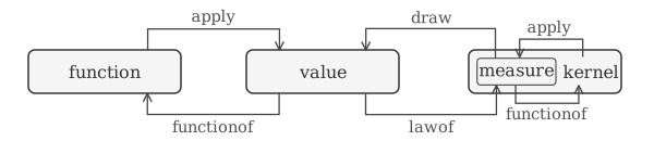
A function represents a reified deterministic DAG, either
implicit (built-in) or explicitly constructed. Ordinary function
application y = f(a, b, ...) introduces a
deterministic node y into the graph.
functionof(y) goes in the opposite direction: it
reifies the ancestor subgraph of y as a first-class
function — the backward program slice of y (Weiser, 1981).
Conversely, a probability measure represents a reified
stochastic DAG, either implicit (built-in) or explicit.
x ~ m (equivalent to x = draw(m))
introduces a stochastic node x by drawing a variate
from a normalized measure (i.e. a probability measure)
m. In the other direction,
m = lawof(x) reifies the ancestor subgraph of
x as a probability measure — the law of
x as a random variable. The identity law relating
the two directions is stated under reification to measures below.
draw differs fundamentally from rand: rand
produces a concrete random value, while draw
introduces a stochastic node that represents the existence of a
random value. Applying rand to a measure reified
from a DAG that contains draw nodes resolves those
draws to concrete random values; evaluating a density on the
same measure instead takes those stochastic nodes as inputs to
the density (unless they are marginalized out in the stochastic
graph).
Reifying measure-valued expressions to
kernels. If
functionof is applied to a measure node, it
generates a transition kernel — a measure-generating callable in
FlatPPL — instead of a function. If the measure is normalized,
the resulting kernel is a Markov kernel. For stochastic-phase
m, functionof(m, ...) reifies the
conditional kernel and functionof(lawof(m), ...)
the marginal (see reification to
measures); for fixed or parameterized phase the two
coincide.
So functionof reifies a value or measure node in
the computational graph to a value function or transition
kernel. While lawof reifies a value node in the
computational graph to a probability measure, and a measure node
to the law of a draw from it (see below).
kernelof (see below) combines lawof
and functionof.
4.8.1 Reification to measures #
lawof(x) reifies the ancestor sub-DAG of
x as the probability measure that
is the total law of x — the probability measure that
x, considered as a random variable, is distributed
according to.
Identity law. lawof(draw(m)) is
equivalent to m for m of fixed or
parameterized phase; for stochastic-phase m it is
the marginal law of a draw from m. Equal laws do
not make values interchangeable as joint components: a
joint of two reified laws of the same draw is the
singular diagonal joint. Otherwise joint(m, m)
contributes a fresh coordinate per occurrence, so the two draws
are independent given m’s stochastic ancestors —
which remain shared — and independent outright when
m has none.
lawof also accepts a measure argument:
lawof(m) is lawof(draw(m)), the law of
a draw from m. Each draw from m is a
fresh coordinate, while the draw nodes among
m’s ancestors remain the same nodes of the trace. A
probability measure of fixed or parameterized phase is its own
law, so lawof(m) is equivalent to m
and lawof is idempotent. For stochastic-phase
m — a random measure — lawof(m) is the
marginal law of a draw from it: the mixture of
the kernel carrying
m’s draw ancestors to m,
over their joint law — the
same integral as kchain.
lawof(m) requires m’s
%mass to be %normalized (see total-mass classes); any other
settled class — %null, %finite,
%locallyfinite, or %unknown — is a
static error, since an unnormalized measure is not its own law.
%deferred is an inference state, not a total-mass
class, and triggers no error; an engine that admits a
%deferred-mass argument assumes normalization
rather than proving it, and must leave the result’s
%mass %deferred. lawof
never normalizes its argument; normalize(m) states
that intent. On a non-nullary kernel, lawof lifts
pointwise, as the uniform kernel
extension does for measure-algebra operations.
Trace of the reified law. A reified measure
or kernel carries its traced sub-DAG as part of its value; a
stochastic node shared between the traces of several joint components enters the
composed trace once.
Phase of the reified law. Although the
ancestor subgraph of the argument of lawof will
typically include stochastic nodes, the resulting measure is
itself deterministic (of parameterized or fixed phase):
lawof absorbs stochasticity into the reified law
rather than propagating it outward. Thus functionof can reify
subgraphs that include stochastic nodes as long as they are
reified to measures (see below).
4.8.2 Reification to functions and kernels #
When called with a single argument (without boundary
specifications, see below), functionof traces the
ancestor subgraph of its argument back to all leaves of
parametric phase — that is, all elementof leaves.
These leaf nodes become the inputs of the reified callable (a
function or a kernel). Fixed ancestors (including
external(...) and load_data(...)
nodes) are resolved to their values and do not become
inputs.
functionof can be called with additional keyword
arguments to designate and label boundary nodes, stopping the
graph trace there — so these nodes become, under their new
names, the inputs of the resulting function or kernel. Boundary
inputs themselves may be of parametric or stochastic phase, but
not fixed phase. functionof effectively substitutes
each boundary node a with an input node
elementof(valueset(a)) under the given name.
FlatPPL has no closures: a reified callable captures no enclosing environment, and a fixed ancestor is resolved to its value rather than retained as a binding.
Referential transparency is a core property of FlatPPL. This
requires that the sub-graph to be reified by
functionof must not contain stochastic nodes that
are not reified to measures. This means that the sub-graph must
not contain draw nodes and nodes derived from them
which are not ancestors of lawof nodes in that
subgraph (since lawof absorbs stochastic phase).
lawof nodes in the sub-graph of a
functionof only operate within that subgraph,
including marginalization.
Consider a simple deterministic computation:
c = a ^ 2
d = max(b, 1.5)
e = c * d
Here e is a specific value during any given
evaluation of the code. But the computation that produces
e from a and b is useful
in its own right: we might want to apply it elementwise over
arrays, or use it as a transformation in pushfwd.
The name e refers to a value, not to the
computation that produced it, so we need a way to extract the
computation as a first-class function:
f = functionof(e)                   # f: {a, b: Real} → Real
C = broadcast(f, a = A, b = B)      # apply f elementwise over arrays A, B
functionof(e) captures the entire computation
leading to e — the sub-DAG that contains
e and all its ancestors — as a reusable function
object. The sub-DAG must be fully deterministic and so must not
contain any draw nodes.
The argument names of the resulting function are the names of the leaf nodes of the reified sub-DAG; the input nodes of the function are decoupled from these leaf nodes. Fixed ancestor nodes are resolved to their values and not exposed as inputs. As the graph nodes are not ordered, the function only supports keyword arguments, not positional arguments.
The output type of the reified function matches the type of
the argument of functionof:
f = functionof(e)                                    # scalar output
f = functionof(record(x = something, y = other))     # record output
f = functionof([something, other])                    # array output
f = functionof((something, other))                   # tuple output
Boundary inputs may also be tuples
(functionof(..., t = some_tuple_expr)), in which
case the reified function takes a tuple argument.
Specifying reification boundaries. Sometimes
only a selected part of the ancestor sub-DAG should be reified.
In our example, e depends on c and
d, which in turn depend on a and
b. If we want the function represented by the
subgraph that starts at a and d —
ignoring how d was computed from a and
b — we can specify boundary inputs that
stop the ancestor backtrace early:
g = functionof(e, p = a, q = d)     # g: {p, q: Real} → Real
M2 = pushfwd(g, some_measure)       # transform a measure over (p, q)
The keyword arguments p = a, q = d declare that
the trace stops at nodes a and d,
which become the inputs of g under the new names
p and q. The computation from
a and b to d is excluded
— g only contains the path from a and
d to e.
Boundary input specification is all-or-none: either every
reified input is specified explicitly, or none is. Boundary
input names must be distinct — a repeated name is a static
error, which likewise forbids a lambda or named function from repeating an
argument name. With explicit boundary specification, the reified
function supports positional arguments in addition to keyword
arguments, with positional order determined by the order in
which boundary inputs are specified. Without a boundary
specification, inputs are traced back to the parameterized-phase
ancestor leaves of the reified expression
(i.e. elementof nodes). Fixed-phase ancestors
(e.g. external and load_data) are
resolved to their values instead. The reified function then only
supports keyword arguments, as no argument order can be
inferred. A specified boundary node a can be
thought of as being substituted with a new node, generated via
elementof(valueset(a)), in the reified graph.
Substitution applies to all boundary nodes before the ancestor
trace runs, so a boundary node whose only paths to the output
pass through another boundary node becomes disconnected from the
output in the substituted graph — the resulting callable is
constant in that input. This is permitted, not an error, and is
what enables hierarchical-model composition (see Kernels and kernelof).
The function argument names do not have to differ from the boundary node names:
h = functionof(e, a = a, d = d) # h: {a, d: Real} → RealThe resulting function h now has arguments named
a and d, but these are local to the
function and decoupled from the original nodes a
and d.
Identity law.
functionof(f(a, b), ..., a = a, b = b, ...) is
equivalent to f.
Lambda notation. A lambda function is a
shorthand notation for functionof with
placeholders. A single-argument lambda is written
arg -> expr; two or more arguments are listed in
parentheses: (arg1, arg2, ...) -> expr (the
single-argument parenthesised form (arg) -> expr
is not valid).
Either form resolves to
functionof(expr', arg1 = _arg1_, ...), where
expr' is expr with every free
occurrence of each arg_i rewritten to the
placeholder _arg_i_. Inside the body,
arg_i refers to the lambda’s input, not to any
module binding of the same name. There is no nullary lambda. A
lambda body must not itself be a lambda: a curried form such as
x -> y -> x + y is a static error under the
placeholder scoping
rule.
For example, x -> 2 * x + 1 is equivalent to
functionof(2 * _x_ + 1, x = _x_), and
(x, y) -> x * y + 1 is equivalent to
functionof(_x_ * _y_ + 1, x = _x_, y = _y_).
4.8.3 Kernels and
kernelof #
kernelof(x, kwargs...) reifies (typically
stochastic) value nodes to Markov kernels. x must
not be a measure. kernelof(x, kwargs...) is
equivalent to functionof(lawof(x), kwargs...)
interpreted within the reified subgraph delimited by
kwargs — the boundary substitution applies before
the inner lawof is interpreted, so an enclosing
kernelof boundary scopes what the inner
lawof marginalizes over.
Identity law.
kernelof(draw(K(a, b, ...)), a = a, b = b, ...) is
equivalent to K. Equal output laws do not make
kernels interchangeable as joint components: a
joint of two reifications of one draw is the
singular diagonal at every input, while a joint of
two constructor kernels contributes a fresh coordinate per
occurrence.
Consider this Bayesian example:
theta1 ~ Normal(mu = 0.0, sigma = 1.0)
theta2 ~ Exponential(rate = 1.0)
a = 5.0 * theta1
b = abs(theta1) * theta2
obs ~ iid(Normal(mu = a, sigma = b), 10)

joint_model = lawof(record(theta1 = theta1, theta2 = theta2, obs = obs))
prior_predictive = lawof(record(obs = obs))
prior = lawof(record(theta1 = theta1, theta2 = theta2))
forward_kernel = kernelof(record(obs = obs), theta1 = theta1, theta2 = theta2)
Here we define
joint_model: the joint probability distribution over parameters and observation.joint_modelis equivalent tojointchain(prior, forward_kernel).prior_predictive: the probability distribution of the observation obtained by marginalizing overtheta1andtheta2— they are internal stochastic nodes in the traced sub-DAG, not boundary inputs, solawofintegrates them out.prior_predictiveis equivalent tokchain(prior, forward_kernel).prior: the probability distribution of the parameterstheta1andtheta2.forward_kernel: the Markov kernel of the forward model; it maps values fortheta1andtheta2to probability distributions of the observation.
The same four objects can be expressed equivalently in pure
measure algebra, without draw or
lawof:
theta1 = elementof(reals)
theta2 = elementof(posreals)
a = 5.0 * theta1
b = abs(theta1) * theta2
obs_dist = iid(Normal(mu = a, sigma = b), 10)

prior = joint(theta1 = Normal(mu = 0.0, sigma = 1.0),
              theta2 = Exponential(rate = 1.0))
forward_kernel = functionof(obs_dist)
joint_model = jointchain(prior, forward_kernel)
prior_predictive = kchain(prior, forward_kernel)
Here forward_kernel is built directly from the
measure-valued expression obs_dist via
functionof (see above), and
joint_model and prior_predictive are
assembled from prior and
forward_kernel using measure combinators.
Reification with interdependent boundary nodes. Reification places no constraint on the DAG-dependency structure among the chosen boundary nodes: a boundary may be an ancestor or descendant of another. Substitution (see reification boundaries) replaces every designated node with a fresh independent input before the ancestor trace runs, so original dependencies between boundaries are erased and the reified callable takes all of them as independent inputs. A boundary whose only paths to the output went through another boundary then has no occurrence in the lowered body — the callable is constant in that input.
The eight-schools model (D. Rubin, 1981) is a typical instance:
mu ~ Normal(0, 5)
tau ~ normalize(truncate(Cauchy(0, 5), interval(0, inf)))
theta ~ iid(Normal(mu, tau), J)
y ~ Normal.(theta, std_errs_data)

prior = lawof(record(mu = mu, tau = tau, theta = theta))
forward_kernel = kernelof(record(y = y), mu = mu, tau = tau, theta = theta)
joint_model = jointchain(prior, forward_kernel)
After substitution, mu, tau,
theta are independent inputs of
forward_kernel. In this specific example
y depends only on theta, so the output
of forward_kernel does not depend on
mu or tau.
Reification and module scope.
functionof and kernelof reify within
the current module only: a parameterized value reached through a
loaded-module reference cannot become an input — neither by the
automatic trace nor as an explicit boundary node — so such a
reification is a static error. A loaded module’s callables and
fixed values may be used in the reified DAG (applied, or
referenced and resolved to their values); only taking a
cross-module parameterized value as an input is disallowed.
Note that lawof reifies a measure, which has no
input list, so it is unrestricted — a measure may reference
cross-module values, keeping the identity law intact across
module boundaries. A reified measure that has a parametric
dependency on a node defined in another module cannot then be
reified to a kernel, due to the restriction above.
4.9 Interface adaptation #
FlatPPL provides relabel for structural renaming
of outputs. At the value level, relabel assigns or
renames fields on scalars, arrays, records, and tables:
v = relabel([1.0, 2.0, 3.0], ["x", "y", "z"])
# equivalent to:
v = record(x = 1.0, y = 2.0, z = 3.0)
and renames record fields and table columns:
v = relabel(record(a = 1.0, b = 2.0, c = 3.0), ["x", "y", "z"])
# equivalent to:
v = record(x = 1.0, y = 2.0, z = 3.0)
and wraps a scalar into a single-field record:
v = relabel(1.0, ["x"])
# equivalent to:
v = record(x = 1.0)
The same output-side renaming lifts directly to sets, functions, measures, and kernels:
named_S = relabel(cartpow(reals, 3), ["x", "y", "z"])
named_f = relabel(f, ["x", "y", "z"])
named_M = relabel(M, ["x", "y", "z"])
named_K = relabel(K, ["x", "y", "z"])
For functions, relabel(f, names) is
post-composition with relabel on the function
result; for measures it is equivalent to
pushfwd(fn(relabel(_, names)), M); for kernels it
acts on the output measures.
See built-in functions for full
reference documentation on relabel.
4.10 Function composition and annotation #
fchain(f1, f2, f3, ...)
composes deterministic functions left-associatively:
fchain(f1, f2, f3)(x) equals
f3(f2(f1(x))).
fchain combines well with auto-splatting: if
f1 returns a record and f2 accepts
keyword arguments matching the record fields, the two functions
compose directly. fchain is the deterministic
analogue of kchain.
bijection(f, f_inv, logvolume)
annotates a function f with its inverse
f_inv and the log-volume-element
logvolume of the forward map. The result is
semantically identical to f, but engines can use
the inverse and volume element when computing densities of
pushforward measures. logvolume may be a function
or a scalar (0 for volume-preserving maps). See pushfwd for
examples.
4.11 Placeholders and holes #
4.11.1 Placeholder variables #
Creating functions and kernels with boundary inputs via
functionof and kernelof requires the
creation of unique global variable names. Placeholder variables
are special variable names of the form _name_
(leading and trailing underscore) that are local to a
functionof(...) or kernelof(...) and
can be thought of as implicitly creating a unique global input
via elementof(anything). All placeholders must
appear both in the expression to be reified and the boundary
input keyword arguments.
For example
f = functionof(_a_ * b + _c_, a = _a_, c = _c_)is equivalent to:
_tmp1 = elementof(anything)
_tmp2 = elementof(anything)
f = functionof(_tmp1 * b + _tmp2, a = _tmp1, c = _tmp2)
Placeholders are not holes (see below). An
expression with placeholders like _a_ * b + _c_
must not appear outside of a
functionof(...) or kernelof(...).
Scoping rule. The scope of a placeholder is
the nearest enclosing functionof or
kernelof. The same placeholder name may appear in
different scopes without conflict:
functionof(functionof(_a_ * b, a = _a_)(some_value) + _a_, a = _a_)A placeholder in an inner functionof or
kernelof must be bound there, so
this code is invalid:
# DISALLOWED:
functionof(functionof(_a_ * b + _c_, a = _a_)(some_value) + _d_, c = _c_, d = _d_)
4.11.2 Holes and
fn #
The reserved name _ denotes a
hole — a position in a deterministic expression
where an argument is not yet supplied. Holes are only valid
inside the special operation fn(...), which
delimits the scope of hole lowering. The form
fn(expr) wraps a hole expression and produces an
anonymous function whose parameters are the holes in
expr, in strict left-to-right reading order. This
is analogous to the
notation used in mathematics to denote a function with a free
argument.
Each _ introduces a distinct positional
parameter, named arg1, arg2, … in
left-to-right reading order. These names are normative and may
be used as keyword arguments. Holes do not inherit keyword names
from enclosing call positions.
Note: Holes work differently than placeholders (see above).
A single hole, resulting in a one-argument function:
neg = fn(0 - _)
poly = fn(polynomial(coefficients = cs, x = _))
The trivial case fn(_) is the identity function,
equivalent to the built-in identity.
Multiple holes — left-to-right positional order:
g = fn(f(_, b, _))
h = fn((_ / _) ^ 2)
Each _ is distinct: fn(_ * _)
multiplies two different inputs rather than squaring one. Use
placeholders if arguments need to appear in the expression more
than once, e.g. functionof(_x_ * _x_, x = _x_).
Lowering. fn(expr) lowers to a
functionof with placeholder variables. For
example
g = fn(f(_, b, _))lowers to
g = functionof(f(_arg1_, b, _arg2_), arg1 = _arg1_, arg2 = _arg2_)which in turn lowers to
_tmp1 = elementof(anything)
_tmp2 = elementof(anything)
g = functionof(f(_tmp1, b, _tmp2), arg1 = _tmp1, arg2 = _tmp2)
4.12 Broadcasting #
broadcast(f_or_K, name = array, ...) or
broadcast(f_or_K, array, ...) maps a function or
kernel elementwise over arrays (and row-wise over tables; see tables). Keyword arguments bind inputs by
name. If the callable has a declared positional order,
positional binding is also permitted.
Dot-syntax. As a concise shorthand for
broadcast, FlatPPL provides dot-call notation
f.(args) and dot-operator notation
a .op b, following the elementwise dotted operators
of MATLAB and the broadcasting dot syntax of Julia.
f.(<args>) lowers to
broadcast(f, <args>) and supports calls with
positional and keyword arguments. So
Normal.(means, sigmas) is syntactic sugar for
broadcast(Normal, means, sigmas). A dotted binary
operator a .op b lowers to
broadcast(opfn, a, b) and a dotted unary operator
.op x to broadcast(opfn, x), where
opfn is the function the plain operator lowers to.
So A .+ B lowers to
broadcast(add, A, B) and .! X lowers
to broadcast(lnot, X). The following examples show
both explicit broadcast calls and the equivalent
dot-notation.
Deterministic broadcast with a named function:
b = 2 * a + 1
f = functionof(b, a = a)
C = broadcast(f, a = A)
b = 2 * a + 1
f = functionof(b, a = a)
C = f.(a = A)With positional argument binding:
C = broadcast(f, A)C = f.(A)Using an anonymous function:
C = broadcast(fn(2 * _ + 1), A)C = fn(2 * _ + 1).(A)Multi-input broadcast:
d = a * x + b_param
g = functionof(d)
E = broadcast(g, a = slopes, x = points, b_param = intercepts)
d = a * x + b_param
g = functionof(d)
E = g.(a = slopes, x = points, b_param = intercepts)Stochastic broadcast — kernel over array, producing an array-valued measure:
K = fn(Normal(mu = _, sigma = 0.1))
D ~ broadcast(K, A)
K = fn(Normal(mu = _, sigma = 0.1))
D ~ K.(A)Return type:
broadcast(function, ...)returns an array value.broadcast(kernel, ...)returns an array-valued measure: the independent product measure of the kernel applications at each array position.
The stochastic case returns a single product measure, not an array of measures. This respects the rule that measures are not stored inside arrays or records while still enabling vectorized stochastic model building.
Independence is explicit: Kernel broadcast means
independent elementwise lifting. It does not cover dependent
sequential kernels, autoregressive chains, or coupled array
structure. For those, use jointchain or
kchain with explicit indexing.
Collection arguments: FlatPPL does not automatically
insert leading or trailing dimensions for array arguments,
unlike some other languages. It does, however, automatically
expand singleton dimensions: All collection arguments (arrays
and tables) must have the same number of axes. Tables count as
having one axis (the table’s rows) here. Along each axis, all
collections must have the same size or be singular (size one).
Size-one array axes are implicitly expanded by repetition to
match the size of the other collection arguments along these
axes. A size-one axis expanded against a zero-length axis yields
length 0. addaxes (see array operations) may be
used to reshape all input arrays to the same number of axes.
For example, given a function f, a matrix
A and a vector b
C = broadcast(f, A, addaxes(b, 1, 0))behaves like NumPy-style broadcasting, while
C = broadcast(f, A, addaxes(b, 0, 1))behaves like Julia-style broadcasting.
Non-collection inputs: Scalar values, functions,
kernels, measures and likelihood objects are allowed as
broadcasting inputs, they are simply not iterated over but held
constant while collection arguments are iterated over. If there
are no collection arguments, broadcast behaves like
a single function or kernel call.
Disallowed inputs: Records and tuples are not allowed as inputs of broadcasts.
Tuple-returning callables: if f returns
a tuple, broadcast(f, ...) returns a tuple of
arrays (componentwise), not an array of tuples.
broadcasted(f) returns a
callable that is equivalent to applying broadcast
to f — that is,
broadcasted(f)(args...) is equivalent to
broadcast(f, args...).
4.13 Reductions #
reduce(f, xs) is a fold over
xs using the binary associative function
f, called positionally as
f(acc, next). For a vector
xs = [x1, x2, ..., xn], it computes
f(...f(f(x1, x2), x3)..., xn). For a table,
xs is traversed row-wise and f takes
two records (the accumulator and the next row). The first
element (or row) is used as the initial accumulator value, so
xs must be non-empty and f must return
a value of the same type as the elements (or rows) of
xs. Since f is required to be
associative, implementations may evaluate in parallel. Unlike
broadcast, reduce accepts only a
deterministic function f, not a kernel.
scan(f, init, xs) is a left
scan over xs using the binary function
f with explicit initial accumulator
init. f is called positionally as
f(acc, next): the running accumulator (of the type
of init) and the next element of xs
(or row record, for tables), returning the new accumulator value
of the same type as init. Output entry
i is f(...f(f(init, x1), x2)..., xi),
i.e. the accumulator after consuming xs[i]; the
result has the same length (or row count) as xs and
does not include init itself. f must
be a deterministic function, not a kernel.
4.14 Multi-axis aggregation #
aggregate(f_reduction, output_axes, expr)
generalizes vector reductions to multi-axis tensor contraction,
as a generalization of Einstein summation.
aggregate evaluates expr at every
combination of values of its named axes and reduces the
resulting scalars by f_reduction along the axes
that do not appear in output_axes, yielding an
array of the shape declared by output_axes.
f_reduction: an order-invariant vector-to-scalar reduction — i.e. a function wheref_reduction(v)is invariant under permutations ofv. The eligible built-ins aresum,prod,mean,var,std,maximum,minimum,median,lanyandlall.output_axes: an axis list of distinct axis names[.name1, .name2, ...]listing the retained axes in output order. Repeated names are a static error. The empty axis list[]is legal and denotes full reduction to a scalar.expr: an expression in which array indexing may contain axis names, likeA[.i, 1, .j]orget(A, .i, 1, .j). Every axis name inoutput_axesmust occur at least once inexpr; any further axis names occurring inexprare reduced over withf_reduction. All array dimensions indexed with the same axis name must have the same length.
Examples:
A = rowstack([[1, 3, 5], [9, 5, 1]])
B = rowstack([[1, 0], [0, 1], [1, 1]])

# Matrix multiplication
C = aggregate(sum, [.i, .k], A[.i, .j] * B[.j, .k])
# → C = [[6, 8], [10, 6]]

# Weighted sum of squared differences, reducing over .j
w = [1, 2, 1]
D = aggregate(sum, [.i, .k], (A[.i, .j] - B[.j, .k])^2 * w[.j])
# → D = [[34, 25], [114, 113]]

# Column-wise variance of a matrix
V = aggregate(var, [.j], A[.i, .j])
# → V = [32, 2, 8]

# Row-wise sum with one fixed column
S = aggregate(sum, [.i], A[.i, 1])
# → S = [1, 9]

# Product over .j of (A + B) entries: prod-reduction over two matrices
P = aggregate(prod, [.i, .k], A[.i, .j] + B[.j, .k])
# → P = [[36, 24], [100, 108]]
Axis names are lexically scoped to the enclosing
aggregate(...) and are not values; see axis names for the surface rules.
:= notation. As a shorthand for
sum-aggregate, FlatPPL provides
result[.name1, .name2, ...] := expr, equivalent to
result = aggregate(sum, [.name1, .name2, ...], expr).
The bracketed axis list may be empty for full reduction to a
scalar.
So
D[.i, .k] := (A[.i, .j] - B[.j, .k])^2 * W[.j]lowers to
D = aggregate(sum, [.i, .k], (A[.i, .j] - B[.j, .k])^2 * W[.j])and the scalar (full-reduction) case
s[] := A[.i] * B[.i]lowers to
s = aggregate(sum, [], A[.i] * B[.i])aggregate composes cleanly with
functionof as the namespace of axis names is local
to the enclosing aggregate and the namespace of
placeholders is local to the enclosing
functionof:
mymatmul = functionof(
    aggregate(sum, [.i, .k], _A_[.i, .j] * _B_[.j, .k]),
    A = _A_, B = _B_
)
Relationship to broadcasting. Aggregation overlaps with broadcasting when no reduction takes place. For example, given
v = some_vector
A = some_matrix  # with first axis of same length as v
B = addaxes(v, 0, 1)
an aggregation (using singleton-axis indexing)
aggregate(f_reduction, [.i, .j], A[.i, .j] * B[.i, !])is equivalent to
broadcast((a, b) -> a * b, A, B)for every eligible f_reduction that is the
identity on a one-element input; var and
std are undefined over a single element, and
lany and lall require boolean
input.
4.15 Metric-aware Einstein summation #
metricsum(metric, output_axes, expr)
is a metric-aware variant of sum-aggregate for
tensor expressions with upper (contravariant) and lower
(covariant) indices.
Variance-marked axis names are required
inside metricsum: .<name>^
denotes an upper-index and .<name>_ denotes a
lower-index axis (see axis names).
Axis-names with variance markers are lexically scoped to the
enclosing metricsum.
All-contravariant canonical storage. Outside
metricsum, arrays carry no tensor metadata and are
interpreted to contain the elements of the all-contravariant
tensor. So a vector v outside of
metricsum represents , and v[.mu^]
inside of metricsum accesses the stored vector
entries directly. Likewise the array metric stores
the elements of the contravariant tensor . So within
metricsum, the covariant vector
v[.mu_] accesses v transformed via the
metric: , where
is equivalent to the contents of inv(metric).
The metric argument is
interpreted as upper-upper , consistent with the rule
above. It must be a square, symmetric, and invertible rank-2
array. Lower-index access of the metric
(metric[.i_, .j_]) denotes the inverse ; mixed access
(metric[.i^, .j_]) denotes the Kronecker delta
.
Output variance specifies the variance of
the components computed by expr, not the
stored layout. The actual result returned by
metricsum is automatically raised to all-upper
canonical storage. Reading the result later inside another
metricsum with the same metric recovers the
originally defined components.
:= notation. As a shorthand,
metric: result[output_indices...] := expr lowers to
result = metricsum(metric, [output_indices...], expr).
Expression restrictions. metric
itself and all arrays indexed with co-/contravariant axis names
in expr must be arrays of scalars.
expr must produce scalar values for all
combinations of axis index values.
Static checks. Every repeated non-output
index in expr must occur exactly twice — once upper
and once lower; every output index must occur in
expr with the same variance and may not also be
contracted; bare neutral aggregate axes (.i without
a variance marker) are not allowed inside
metricsum. A non-output index occurring once is
legal and is summed over by the lowering below. Its variance is
therefore semantically significant, and the result is
coordinate-dependent rather than tensorial.
Equivalence to aggregate under identity
metric. metricsum(eye(n), ...) is
equivalent to an aggregate(sum, ...) with
co-/contravariant axis names replaced by aggregate
axis names.
Lowering to aggregate. Each
_ (lower-variance) axis name in expr
becomes an inv(metric) contraction; each
_ output axis becomes a metric
contraction after the sum, raising the result to all-upper
canonical storage. The whole lowering may be expressed as a
single aggregate(sum, ...) with metric factors
inlined, or as a chain that precomputes mixed-variance
intermediates as common subexpressions; both forms are
semantically equivalent.
Example. Composition of three Lorentz
transformations as (1,1)-tensors, under metric
g:
g: L[.mu^, .rho_] := L1[.mu^, .nu_] * L2[.nu^, .sigma_] * L3[.sigma^, .rho_]Equivalent non-shorthand form:
L = metricsum(g, [.mu^, .rho_],
    L1[.mu^, .nu_] * L2[.nu^, .sigma_] * L3[.sigma^, .rho_])
Lowering to aggregate, inline metric
insertion:
__g_down = inv(g)
L = aggregate(sum, [.mu, .rho_up],
    L1[.mu, .a] * __g_down[.a, .nu] *
    L2[.nu, .b] * __g_down[.b, .sigma] *
    L3[.sigma, .c] * __g_down[.c, .rho] *
    g[.rho, .rho_up]
)
Lowering to aggregate, precomputed
mixed-variance intermediates:
__g_down = inv(g)
__L1_mixed = L1 * __g_down
__L2_mixed = L2 * __g_down
__L3_mixed = L3 * __g_down
__L_mixed = aggregate(sum, [.mu, .rho],
    __L1_mixed[.mu, .nu] * __L2_mixed[.nu, .sigma] * __L3_mixed[.sigma, .rho]
)
L = __L_mixed * g
4.16 Lowered linear form #
A FlatPPL module admits a stable lowering to a linear
SSA-style core form in which every non-atomic subexpression is
bound to an auto-generated unique name (see Placeholders and holes for
the lowering stages). In the resulting form, every binding’s
right-hand side is either a literal or a function call:
name = c or name = f(name, ...).
Operators, indexing, field access, and array literals all
desugar to function calls (add, get,
vector, etc.), giving the core form a uniform
shape. This is a semantic property of FlatPPL modules; it is
independent of the surface syntax.
4.17 Standard modules #
FlatPPL’s core built-ins aim to be domain-neutral.
Functionality and vocabulary more specific to particular
disciplines is provided via standard modules that are not part
of base.
Standard modules are versioned independently from FlatPPL
itself, and loaded via
standard_module(name, compat). The
names of standard modules are official and coordinated;
compat is a compatibility version string with the
same semantics as flatppl_compat
(see below). standard_module only accepts
positional arguments, not keyword arguments.
For example:
hepphys = standard_module("particle-physics", "0.1")
peak = hepphys.CrystalBall(m0 = 125.0, sigma = 2.0, alpha = 1.5, n = 3.0)
See section Standard modules for the current set of FlatPPL standard modules.
Engine support. FlatPPL engines are not required, but encouraged, to implement all standard modules if feasible on the given platform.
4.18 Module composition #
A FlatPPL module is a flat namespace of named bindings (see above). Modules can load other modules written in FlatPPL though, to make models composable:
load_module(source) loads a
FlatPPL file and returns a module reference.
source may be a file path or a URL (see Remote file caching).
Each load_module call instantiates the loaded
module independently: two calls share no nodes, even with
identical source and substitutions, so reified
callables from different calls have disjoint stochastic
ancestors. To share one instance, bind the module reference once
and reuse the name.
In the canonical syntax, bound names in the loaded module are accessed via dot syntax:
sig_module = load_module("signal.flatppl")
bkg_module = load_module("background.flatppl")

sig_model = sig_module.model
bkg_model = bkg_module.model
Access to loaded modules is not transitive: The loading
module may access names in the loaded module, but not names in
modules loaded by that module, so sig_module.model
is valid but sig_module.some_other_module.some_name
is not.
Load-time substitution.
load_module may also be called with keyword
arguments to substitute explicit input nodes of the loaded
module:
sig_module = load_module("signal_channel.flatppl", mu = signal_strength, theta = nuisance)The left-hand side of each keyword argument must refer to an input of the loaded module. The phase of this input determines what it can be bound to on the right-hand side:
externalinputs of the loaded module may only be bound to fixed values in the loading module.elementofinputs of the loaded module may only be bound to parameterized values in the loading module.- No other kinds of nodes in the loaded module may be bound to nodes in the loading module.
Value sets must be compatible in both cases, so the computational structure of the loaded module is not modified.
Stochastic boundary. Only bindings of
fixed or parameterized phase in the
loaded module are accessible from the loading module
(module.name). Bindings of stochastic
phase — direct draws or values with draw ancestors
that have not been reified via
lawof/kernelof — are invisible to the
loading module. This preserves referential transparency and
avoids semantic ambiguity when two loaded modules load a common
third module.
Path resolution. Relative file paths in
load_module(...) are resolved relative to the
directory of the FlatPPL file containing that
load_module(...) call, not the host process’s
working directory. For embedded FlatPPL code, relative paths are
resolved relative to the directory of the source file containing
the embedded FlatPPL code block. The forward slash
/ is the mandatory path separator on all platforms.
Parent-directory traversal via .. is allowed.
Absolute file paths are permitted but discouraged, as they
prevent relocatable model repositories.
Aliasing is just assignment:
sig_model = sig_module.model creates a local alias
— a reference to the same underlying object in the loaded
module’s DAG, not a clone.
Bundles. source may be a bundle
holding a main FlatPPL module file and its module and data
dependencies. If source is a directory,
load_module loads its root
main.flatppl (which will typically itself use
load_module and load_data to load
dependencies located under that directory). If
source is a ZIP file (extension .zip;
.flatppl.zip recommended where practical), it loads
main.flatppl from the archive root. If there is no
root main.flatppl in the archive, but the archive’s
sole top-level entry is a directory containing a
main.flatppl, it is loaded from there. A missing
main.flatppl is an error.
Within a bundle (directory or ZIP), relative paths — in both
load_module and load_data — resolve
only inside the bundle and must not escape its root via
...
4.19 FlatPPL version compatibility #
A FlatPPL module may declare which versions of FlatPPL it is
compatible with via the reserved binding
flatppl_compat:
flatppl_compat = "0.1"The value is a string following Julia-style semantic
versioning conventions: for pre-1.0 versions, the minor version
is breaking ("0.1" means 0.1.0, 0.2.0); for versions 1.0, the major version is
breaking ("1" means 1.0.0, 2.0.0). Multiple ranges are
comma-separated and combined with OR:
flatppl_compat = "0.8, 0.9.2, 1.0.0, 2"declares compatibility with versions v0.8.x, v0.9.2 up to (excluding) v0.10, v1.x.y, and v2.x.y.
The declaration is optional. Short-lived models, didactic examples and the like may omit it. For embedded FlatPPL blocks, version compatibility may be managed at the host-language level (e.g. via Python or Julia package/environment dependency version bounds on FlatPPL packages). FlatPPL files of models intended for long-term use, publication or archival should definitely include a compatibility declaration.
The compatibility declaration of a loaded module is
accessible via dot syntax (like any other bound value in the
module): some_module.flatppl_compat.
4.20 Code documentation #
FlatPPL treats documentation as a first-class property of
bindings, not as ambient commentary.
Doc-comments in surface FlatPPL
(%, %%%; see section Syntax) attach to bindings and are
preserved when lowering to FlatPIR.
Default markup and markup tags. By default, documentation is written in Markdown. The markup language can be explicitly selected with a markup tag. FlatPPL tooling should know how to handle the following tags:
%md/%%%md: GitHub-Flavored Markdown with math ($...$,$$...$$)%typ/%%%typ: Typst
Markup tags should reflect the canonical file extension of the markup language.
Attachment. A doc-comment attaches to at most one binding, in one of two positions:
- Leading: before a FlatPPL binding (only whitespace,
newlines and
;statement separators between). - Trailing: a single-line
% ...after a binding’s right-hand side, before the next newline or;statement separator. Block%%%forms must not be in trailing position.
Each binding may carry at most one doc-comment (leading or
trailing, not both). Two leading % ... lines on the
same binding are an error — use a %%% block for
multi-line content. A doc-comment that doesn’t attach to a
binding is invalid code.
Module-level documentation. A doc-comment
attached to the flatppl_compat binding serves to
document the module itself:
%%%
# Eight-schools model

Hierarchical Normal model after Rubin (1981).
%%%
flatppl_compat = "0.3"
Comments are not documentation. Plain
comments (#, ###) are discarded at
parse time and do not appear in FlatPIR. They are
author-eyes-only notes on the surface source. Anything intended
to outlive the surface file — for tools, for downstream readers
via FlatPIR, or for export to external systems — must use a
doc-comment. (FlatPIR
has its own ; line comments in the canonical text
syntax, but those are reserved for tooling annotations and do
not carry user-written surface comments.)
4.21 Remote file caching #
A load_module(url) or load_data(url)
source may be an
http/https URL rather than a local
path. FlatPPL is meant to be supported by multiple engines and
tools in a variety of host languages, and the design leaves a
lot of freedom to individual FlatPPL implementations. But
caching of remote content to local files should be consistent
across various tools and engines, so they should adhere to the
following conventions (subject to change in future FlatPPL
versions) and thus use a shared local cache:
Cache directory. The main cache directory
(referred to below as <flatppl-cachedir>) is
set by the environment variable FLATPPL_CACHEDIR.
If not set, the following default is used:
- Linux and BSD: A directory
flatppldirectly under the XDG cache directory (defaults to$HOME/.cache/flatppl). - macOS:
$HOME/Library/Caches/flatppl - Windows:
%LOCALAPPDATA%\flatppl
Layout and keys. Under
<flatppl-cachedir>/v1/:
objects/<kk>/<key>.<ext>holds the fetched URL content.keyis the lowercase-hexadecimal SHA-256 of the request URL with any#-fragment removed (no other normalization), and<kk>is the first two characters ofkey.<ext>is the requested file’s full trailing extension — everything after the first.in the URL’s final path segment — so a multi-part extension is kept whole; a final segment with no.uses just<key>.objects/<kk>/<key>_meta.jsonis a mandatory JSON metadata file with fieldsurl(the original URL),resolved_url(the URL fetched after any redirects),retrieved(ISO 8601 UTC time),content_type, and the HTTP validatorsetagandlast_modified(any may benullif the server omits it). Readers ignore unknown fields.trust/<kk>/<key>is a per-URL trust marker — its presence means the URL is trusted — keyed by the same<kk>/<key>as the object. Trust is based on the original URLs, not on redirect URLs.tmp/holds temporary files during downloads, must be on the same filesystem asobjects/to achieve atomic renames.
The cache is keyed by URL hash; there is no separate index,
and objects/ is its complete state.
Resolve and fetch. To resolve a URL, FlatPPL
implementations use the cached object under the matching hash if
present. Otherwise, implementations check if the URL is trusted
(see below), fetch the URL via the temporary directory (see
below for details), and store the URL content in the objects
directory under the URL hash with the file extension added. URL
redirects are followed for download but the hash of the original
URL is used in the cache. A fetch that fails — a network error,
a final response whose status is not 2xx, or an
unresolvable redirect — is an error, and nothing is written to
the cache (no partial object and no metadata). If
FLATPPL_CACHE_OFFLINE is set, a cache miss is an
error and no URL fetch is attempted.
Trust. Before fetching a URL that has no
trust marker, interactive tooling must obtain the user’s
approval and then create its
trust/<kk>/<key> marker.
Non-interactive tooling must error if a requested URL is not
marked as trusted. If the environment variable
FLATPPL_TRUST is set, all URLs are trusted
implicitly by interactive and non-interactive tooling, but no
trust markers are created.
Atomicity and concurrent tools. Content is
initially downloaded to the tmp/ directory, then
fsynced and then atomically renamed into the destination file
under the objects directory. The _meta.json file is
written the same way and renamed into place before its content
object, so a present <key>.<ext> always
has its metadata. Trust markers are created with an exclusive
O_CREAT | O_EXCL open. The whole cache is lock-free
and <flatppl-cachedir> should be located on a
file system that supports atomic renaming.
Environment variables.
| Variable | Effect |
|---|---|
FLATPPL_CACHEDIR |
Override the cache directory; used verbatim. |
FLATPPL_CACHE_OFFLINE |
Never fetch — a cache miss is an error. |
FLATPPL_TRUST |
Trust all URLs implicitly (no prompt; no trust markers created). |
5 Canonical syntax #
This section specifies the canonical surface form of FlatPPL, used throughout this document as a notation for defining FlatPPL semantics and presenting examples. It also defines a mechanism for embedding FlatPPL in Python and Julia (see host-language embedding below).
The semantics of FlatPPL do not depend on this canonical syntax. Alternative syntactical representations may be advantageous for specific software ecosystems and use cases. Such alternative representations must map directly to and from canonical FlatPPL without change in semantics.
Canonical FlatPPL uses the filename extension
.flatppl.
5.1 Statements #
A FlatPPL module is a sequence of statements separated by newlines or semicolons (equivalent). One statement per line is the recommended style; semicolons exist primarily as a fallback for channels that may not preserve line breaks.
5.2 Comments #
# starts a line comment; ### alone
on a line opens a block comment closed by a matching
### alone on a line. Both forms are discarded by
the parser. Line comments are terminated by the next newline or
;, whichever comes first. Block fences may have
leading horizontal whitespace (so embedded FlatPPL inside an
indented host block is fine).
x = 3.14  # Inline comment.

###
Block comment.
###
For documentation that attaches to bindings and survives into FlatPIR, see below.
5.3 Documentation #
Doc-comments are lexically symmetric to plain comments
(% ↔︎ #, %%% ↔︎
###) but attach to bindings and survive into FlatPIR. Semantics,
attachment rules, default markup, and module-level documentation
are specified in Code
documentation; this section covers the surface lexical forms
only.
- Single-line:
%[<markup>]? <content>runs to end of line or to the next;, whichever comes first. - Block:
%%%[<markup>]?alone on a line opens; a matching%%%alone on a line closes. Content is verbatim, line by line. Fence lines may have leading horizontal whitespace, which is ignored; content lines are taken as written. - Markup tag (optional, no space after the
leading
%/%%%):md(default, GitHub-Flavored Markdown with$...$/$$...$$math) ortyp(Typst). An unrecognized tag is a parse error. The naming convention is “typical file extension”; additional tags may be added in future spec versions.
% Prior mean.
mu = 0

sigma = 1  % Prior std. dev.

%%%
The observation model: independent Gaussians, shared unknown scale.
%%%
obs ~ iid(Normal(mu, sigma), 5)
5.4 Supported constructs #
FlatPPL has a very lean syntax:
- Bindings:
name = exprand decompositiona, b, c = expr(see below). - Tilde bindings:
name ~ exprand decompositiona, b ~ expr, equivalent toname = draw(expr)anda, b = draw(expr)respectively (see variates and measures). - Named functions:
f(arg1, arg2, ...) = expris shorthand for bindingfto a lambda (see named functions). - Literals: numbers (
3.14,42,0xF7,0x3e,1_000_000,1.45e7), strings ("foo"), booleans (true,false), arrays ([1, 2, 3]), records (record(a = 1, b = 2)), tuples ((a, b)). - Infix arithmetic, exponentiation, and
comparisons:
+,-,*,/,^, unary-, and the comparisons<,>,==,!=,<=,>=, andin(set membership). Comparisons may be chained:a < b <= clowers toland(a < b, b <= c).^is right-associative and binds tighter than unary-. - Logical operators:
&&,||,!(lowering toland,lor,lnot; see Logic and conditionals). - Broadcasting: Dot-call
f.(...)and dot-prefixed operator applicationa .+ bare syntactic sugar forbroadcast(see Broadcasting syntax). - Lambda:
arg -> expr(single arg) or(arg1, arg2, ...) -> expr(multi-arg) is shorthand forfunctionofwith placeholders (see Lambda syntax). - Aggregation: axis-indexed binding
C[.i, .k] := expris shorthand for sum-aggregate; the metric-prefixed formg: C[.mu^, .nu_] := expris themetricsumshorthand for metric-aware Einstein summation. (See Axis names and aggregation.) - Function calls:
f(x, y)(positional),f(a = x, b = y)(keyword) andf(object, a = x, b = y)(for some special operations). - Indexing and field access:
A[i],A[i, j],A[:, j],r.field.
Also see the formal grammar below.
See binding names for rules
on binding names, name resolution, and the reserved modules
self and base.
5.5 Excluded constructs #
The above are the only syntactical constructs allowed in FlatPPL. The following Python and Julia constructs, for example, are not allowed directly in canonical FlatPPL, but can easily be represented in other ways:
- No type annotations. Types are inferred from the semantic rules.
- No loops or conditionals. Use
ifelse(cond, a, b)for piecewise definitions (see logic and conditionals). - No function definition blocks. A function
body is a single expression (a lambda or
f(x) = expr, see named functions); for named intermediate steps usefunctionof(see language design). - No implicit operator broadcasting. Infix
+,-,*,/,^and unary-follow standard linear-algebra and scalar semantics:+and-require operands of identical shape (scalars, or arrays of matching shape),*supports the products enumerated in operator-equivalent functions,/requires a scalar divisor, and^is scalar-only.
5.6 Decomposition syntax #
The left side of an = or ~
assignment may decompose an array, record, or tuple into named
components:
a, b, c ~ MvNormal(mu = mean_vector, cov = cov_matrix)
# equivalent to
# a, b, c = draw(MvNormal(mu = mean_vector, cov = cov_matrix))

x, y = some_record
l, m, n = some_tuple
value, _ = rand(rstate, m)
Decomposition is by position. For records, the field order determines which value each name receives; for arrays and tuples, positional index does. This is syntactic sugar: it lowers to an assignment followed by indexed or field-access bindings.
5.7 Indexing and slicing #
FlatPPL uses 1-based indexing.
A[:, j] selects all elements along the first
axis at fixed index j. This lowers to
get(A, all, j), where all is a
predefined selector meaning “entire axis.”
A[:, j]          # → get(A, all, j)
A[i, :]          # → get(A, i, all)
T[:, :, k]       # → get(T, all, all, k)
T[i, :, k]       # → get(T, i, all, k)
! is the only selector: it extracts
the unique element of a length-1 axis. This lowers to
get(A, only, ...). The indexed axis must have
length one.
A[!, j]          # → get(A, only, j)
v[!]             # → get(v, only)
5.8 Special operations #
elementof(S), valueset(x),
draw(M), lawof(x),
functionof(...), kernelof(...), and
fn(...) are special operations with their own
syntax rules — they are not ordinary function calls. Their
semantics are defined in language
design. load_module(...) is documented in multi-file models.
5.9 Broadcasting syntax #
FlatPPL provides dot-prefixed shorthand for broadcast:
f.(<args>)— dot-call.a .op b— dotted binary operators..op x— dotted unary operators.
Each dotted operator has the same precedence as its plain
counterpart. in has no dotted form (its right
operand is a set, not a broadcastable value). See Broadcasting for dot-notation
lowering.
5.10 Lambda syntax #
Lambda functions, denoted as arg -> expr and
(arg1, arg2, ...) -> expr, are syntactic sugar
for functionof.
(arg) -> expr is not legal syntax (no
parentheses around the argument in single-argument lambdas). At
least one argument is required (no nullary lambdas).
The body extends as far right as possible — lambdas have
lower precedence than every other expression form, so
(a, b) -> a^2 + b^2 parses with
a^2 + b^2 as the body. Inside the body, the
argument names refer to the lambda’s inputs and shadow any
module-level binding of the same name. See Reification to functions and kernels
for the desugaring.
5.11 Named functions #
f(arg1, arg2, ...) = expr is syntactic sugar for
binding f to a lambda
— it desugars to f = (arg1, arg2, ...) -> expr.
As for lambdas, at least one argument is required
(f() = expr is not legal; bind a plain value with
f = expr) and the argument names are local to the
body. The defined function accepts positional and keyword calls,
and f is a first-class value usable wherever a functionof result
is.
f(x, y) = x^2 * y^2                          # equivalent to f = (x, y) -> x^2 * y^2
g(x, y, z) = record(p = x + y, q = y * z)    # record/array/tuple body → multi-output
h(x, y) = [x / y, x * log(y)]
The construct is purely a surface rewrite: it adds no FlatPIR node and
inherits every function property — scoping, duplicate-argument
rules, phase, doc-comment attachment — from the lambda
desugaring. There is no tilde form, since a measure is not a
function (f(arg1, ...) ~ expr is not legal).
5.12 Axis names and aggregation #
Axis names are written .<name> and are
symbolic index labels used by aggregate. They are
lexically scoped to the enclosing aggregation and are not
values: an axis name is legal only as an entry in
aggregate’s output_axes axis list, as
an index inside [...] within the body, or as a
binder on the left-hand side of :=. Used anywhere
else it is a static error.
The aggregation form C[.i, .j, ...] := expr is
shorthand for sum-aggregate; see there for
the desugaring. The bracketed axis list may be empty
(x[] := expr) for full reduction to a scalar.
Axes may carry a variance marker —
.<name>^ (upper / contravariant) or
.<name>_ (lower / covariant) — inside metricsum for
metric-aware Einstein summation. The marker form
metric: C[...] := expr is the shorthand for
metricsum. Axis names themselves may not end in
_, since trailing _ is reserved as the
lower-variance marker.
5.13 Host-language embedding #
FlatPPL defines a recommended mechanism for embedding FlatPPL code in Python and Julia. Python and Julia implementations of FlatPPL should use this approach so that independent tooling, like FlatPPL grammars and extensions for code editors, can support it consistently.
Embedding FlatPPL in Python should be
realized via a call to a function flatppl on a raw
string, flatppl(r"""<FlatPPL code>"""),
e.g.
model = flatppl(r"""
mu = elementof(reals)
x ~ Normal(mu = mu, sigma = 1)
""")
FlatPPL is not indentation-sensitive, so leading horizontal whitespace from an indented Python block does not affect the model.
Embedding FlatPPL in Julia should be
realized via a Julia string macro
flatppl"""<FlatPPL code>""", e.g.
model = flatppl"""
mu = elementof(reals)
x ~ Normal(mu = mu, sigma = 1)
"""
Host data enters an embedded model only through the explicit
input mechanisms (external, load_data,
and parameterized load_module); embedded FlatPPL
does not capture host-language variables, and host string
interpolation should not be used to splice values into a model,
as that would bake constants into the graph instead of creating
input nodes.
The only sequence that cannot appear inside embedded FlatPPL
source — including inside doc-comments — is a literal
""", which would terminate the host string.
Markdown fenced code inside doc-comments should use
triple-backticks (```).
5.14 Formal grammar #
The canonical surface syntax is defined in EBNF below (ISO
14977-style, with ::= for production and
| for alternation).
Grammar.
(* Top level *)
Module          ::= StmtSep* (Statement (StmtSep+ Statement)*)? StmtSep* EOF
Statement       ::= Binding | TildeBinding | Decomposition | TildeDecomposition
                  | FunctionDefinition
                  | AggregateBinding | MetricsumBinding

(* Bindings *)
Binding            ::= Name "=" Expression
Decomposition      ::= Name ("," Name)+ "=" Expression
TildeBinding       ::= Name "~" Expression
TildeDecomposition ::= Name ("," Name)+ "~" Expression
FunctionDefinition ::= Name "(" Name ("," Name)* ")" "=" Expression
AggregateBinding   ::= Name AxisList ":=" Expression
MetricsumBinding   ::= Name ":" Name AxisList ":=" Expression

(* Expressions — lambda at top, logical OR/AND above comparisons,
   exponentiation below multiplicative *)
Expression      ::= Lambda | Or
Lambda          ::= LambdaParams "->" Expression
LambdaParams    ::= Name | "(" Name "," Name ("," Name)* ")"
Or              ::= And (("||" | ".||") And)*
And             ::= Comparison (("&&" | ".&&") Comparison)*
Comparison      ::= Additive (CompOp Additive)*       (* chained *)
Additive        ::= Multiplicative (AddOp Multiplicative)*
Multiplicative  ::= Unary (MulOp Unary)*
Unary           ::= ("-" | ".-") Unary | ("!" | ".!") Unary | Exponential
Exponential     ::= Postfix (("^" | ".^") Unary)?
Postfix         ::= Primary (FieldAccess | DotCall | Indexing | Call)*
Primary         ::= Literal | Name | Axis | AxisList | "(" Expression ")"

FieldAccess     ::= "." Name
DotCall         ::= "." "(" CallArgs ")"
Indexing        ::= "[" IndexExpr ("," IndexExpr)* "]"
IndexExpr       ::= Expression | ":" | "!"
Axis            ::= "." AxisName VarianceMarker?
AxisName        ::= Letter
                  | Letter (Letter | Digit | "_")* (Letter | Digit)
                    (* Identifier that must not start with "_" or end with "_";
                       trailing "_" is reserved as the lower-variance marker. *)
VarianceMarker  ::= "^" | "_"
AxisList        ::= "[" (Axis ("," Axis)*)? "]"

CompOp          ::= "<" | ">" | "==" | "!=" | "<=" | ">=" | "in"
                  | ".<" | ".>" | ".==" | ".!=" | ".<=" | ".>="
AddOp           ::= "+" | "-" | ".+" | ".-"
MulOp           ::= "*" | "/" | ".*" | "./"
ContinuationOp  ::= AddOp | MulOp | CompOp | "^" | ".^"
                  | "&&" | "||" | ".&&" | ".||"
                  | "->" | "=" | "~" | ":=" | ":"
                    (* Every infix binary operator, the lambda arrow, and the
                       binding operators. Only a TRAILING occurrence continues a
                       line (see "Statement separation"); a line beginning with
                       an operator starts a new statement, and is a parse error
                       unless that operator is unary. *)

(* Calls *)
Call            ::= "(" CallArgs ")"
CallArgs        ::= PositionalArgs | KeywordArgs | MixedArgs
PositionalArgs  ::= Expression ("," Expression)*
KeywordArgs     ::= KeywordArg ("," KeywordArg)*
KeywordArg      ::= Name "=" Expression
MixedArgs       ::= Expression ("," Expression)* ("," KeywordArg)+

(* Literals *)
Literal         ::= Number | String | Boolean | ArrayLiteral | RecordLiteral | TupleLiteral
Boolean         ::= "true" | "false"
Number          ::= IntegerLit | RealLit
ArrayLiteral    ::= "[" Expression ("," Expression)* ","? "]"
RecordLiteral   ::= "record" "(" KeywordArg ("," KeywordArg)* ","? ")"
TupleLiteral    ::= "(" Expression "," Expression ("," Expression)* ","? ")"

(* Lexical *)
Name            ::= (Letter | "_") (Letter | Digit | "_")*
IntegerLit      ::= DecIntLit | HexIntLit
DecIntLit       ::= Digit ("_"? Digit)*
HexIntLit       ::= "0x" HexDigit ("_"? HexDigit)*
HexDigit        ::= Digit | "a" .. "f" | "A" .. "F"
RealLit         ::= DecIntLit "." DecFracPart? Exponent?
                  | DecIntLit Exponent
                  | "." DecFracPart Exponent?
DecFracPart     ::= Digit ("_"? Digit)*
Exponent        ::= ("e" | "E") ("+" | "-")? DecIntLit
String          ::= '"' StringChar* '"'
StringChar      ::= any character except '"' and '\' | '\' EscapeChar
EscapeChar      ::= '"' | '\' | "n" | "t" | "r" | "0"
Letter          ::= "a" .. "z" | "A" .. "Z"
Digit           ::= "0" .. "9"
Newline         ::= LF | CR | CRLF
StmtSep         ::= Newline | ";"

(* Plain comments — discarded by the parser *)
LineComment     ::= "#" { any character except newline or ";" }
BlockComment    ::= HWS* "###" HWS* Newline
                    { any line whose trimmed content is not "###" }
                    HWS* "###" HWS* Newline

(* Doc-comments — attached to bindings; see "Documentation" *)
DocLine         ::= "%" MarkupTag? { any character except newline or ";" }
DocBlock        ::= HWS* "%%%" MarkupTag? HWS* Newline
                    DocBlockLine*
                    HWS* "%%%" HWS* Newline
DocBlockLine    ::= { any character except newline } Newline
                  ; a line whose trimmed content equals "%%%" closes the block
MarkupTag       ::= "md" | "typ"
HWS             ::= " " | "\t"            (* horizontal whitespace *)
Statement separation. Statements are
separated by one or more newlines or semicolons; the two are
fully equivalent. Blank lines and comment-only files are
permitted. Newlines inside an unclosed ( or
[ (paren/bracket depth > 0) are treated as
whitespace (implicit line continuation), letting expressions
span multiple lines:
rate = superpose(
    weighted(mu_sig * efficiency, signal_template),
    bkg_template
)
At paren/bracket depth 0, a newline is likewise treated as
whitespace when the line’s last token is a
ContinuationOp, so the statement continues on the
next line that carries a token. A trailing line comment, and any
blank or comment-only lines in between, do not end the
continuation. A ^ or _ immediately
following an axis name is that axis’s
variance marker, not a ContinuationOp.
rate = mu_sig * signal_yield +      # trailing operator continues the line
       mu_bkg * bkg_yield
Note on MixedArgs.
Syntactically, any Call may use
MixedArgs (one or more leading positional
expressions followed by one or more keyword arguments).
Semantically, only the special operations
functionof, kernelof,
broadcast, load_module, and
load_data accept this shape; other callables must
use PositionalArgs or KeywordArgs
only. Among these, functionof,
kernelof, load_module, and
load_data take exactly one leading positional
argument; only broadcast accepts multiple
positional arguments before the keyword arguments.
Note on reserved words. The keywords
in, true, false,
all, and only are recognized before
Name and cannot be used as bindings. The top-level
binding names inputs and outputs are
reserved for the determinization
signature.
Note on holes and placeholders. The lexical
rule for Name admits _ (the hole used
inside fn(...)) and trailing-underscore identifiers
_x_ (placeholders used inside
functionof/kernelof). The grammar
parses both as ordinary Name; the syntactic
restrictions on where they may appear are documented in functions and reification.
Note on axis names. The grammar admits
Axis (.<name>) as a
Primary, but Axis is legal only inside
an aggregation — as an entry of
aggregate’s output_axes, as an
[...] index in its body, or as a binder of an
AggregateBinding. Anywhere else it is a static
error. The grammar likewise admits AxisList as a
Primary, but it is legal only as the
output_axes argument of an aggregate
or metricsum call and as the axis-list binder of an
AggregateBinding or MetricsumBinding;
anywhere else it is a static error. Unlike
ArrayLiteral, AxisList may be empty:
aggregate(sum, [], expr) denotes full reduction to a scalar.
Note on tuples. (x) is a
parenthesised expression. (x, y) is a tuple. The
single-element form (x,) is not in the grammar —
single-element tuples are not supported (consistent with the
design rule that tuples have at least two components).
Note on parser disambiguation. The grammar
is intended to be parsed with bounded lookahead.
CallArgs is technically ambiguous in pure EBNF (an
Expression can begin with a Name, and
so can a KeywordArg), but a one-token lookahead
after the leading Name (checking for
=) suffices to choose between
PositionalArgs/MixedArgs and
KeywordArgs. After a ., a one-token
lookahead distinguishes DotCall (.
followed by () from FieldAccess
(. followed by a Name). Dot-prefixed
operators (.+, .^, .==,
…) are single tokens, recognized by maximal munch. Maximal munch
also resolves the trailing-dot real literal against a dotted
operator: in 1./x the 1. is the real
literal 1.0 (so this is 1.0 / x), as
in Julia. A dotted operator on an integer-literal operand needs
whitespace or an explicit fractional part — 1 ./ x
or 1.0 ./ x. After a closing ), a
one-token lookahead for -> distinguishes a
Lambda from a parenthesised expression or tuple
literal; a parenthesised lambda is well-formed only if the
parenthesised content was a list of two or more bare
Names. A bare Name immediately
followed by -> is a single-argument
Lambda. At statement level, a Name
followed by ( begins a
FunctionDefinition (no other statement form starts
Name "("), disambiguated by checking that the
closing ) is followed by =. A
.Name token is FieldAccess when it
follows a Postfix-able expression, and
Axis otherwise (at the start of a
Primary). Inside [...], a
! token followed immediately by , or
] is the only axis keyword; otherwise
it is the unary logical-not operator starting an Expression. In
AxisList’s legal positions (as above),
[...] parses as AxisList, not
ArrayLiteral.
6 Measure algebra and analysis #
This section documents the measure-level operations that form the compositional core of FlatPPL.
6.1 Measure-theoretic foundations #
A measurable space is a pair of a set and a -algebra. All spaces arising in FlatPPL are standard Borel spaces (, , and finite products thereof), where the -algebra is the standard Borel -algebra and can be left implicit. A measure on is a -additive function . A probability measure has . All measures in FlatPPL are -finite (admitting a countable cover of finite-measure sets), which ensures that product and marginalization operations are well-defined and that the Radon-Nikodym theorem applies whenever a measure is absolutely continuous with respect to its reference measure (so densities exist). In the rest of this document, “measure” means “-finite measure.”
A transition kernel (or kernel) from to is a measurable function , where is the space of measures on . When each is a probability measure, the kernel is called a Markov kernel. In FlatPPL, kernels are represented as functions that map value points to measures.
The classical Giry monad (Giry, 1982) operates on probability measures, which are normalized. FlatPPL extends this to -finite measures in general, e.g. to represent non-normalized posteriors and intensity measures. Staton et al. (2016) and Staton (2017) provide the formal basis for this extension using the more general class of s-finite measures; all -finite measures are s-finite, so FlatPPL’s algebraic operations are well-founded within that framework.
Density convention. All density formulas in this section are with respect to a reference measure implied by the constituent distribution types: Lebesgue for continuous variates, counting measure for discrete variates. When a kernel is parameterized by , the family is assumed dominated by a single -independent reference measure.
Reference measure for product measures. When
joint(M1, M2, ...) (or iid(M, size),
jointchain(M, K1, ...) etc.) combines components
with individual reference measures (each either
Lebesgue or Counting on the
corresponding component support), the reference measure of the
product is the product on the joint variate space. For
components sharing no stochastic ancestor, the joint density
w.r.t. this product reference is the product of the component
densities; a shared-ancestor joint keeps the same
product reference, with density given by its equivalent record
law (see joint). Mixed
continuous-discrete joints are handled uniformly under this
rule:
e.g. joint(c = Normal(mu = 0, sigma = 1), k = Poisson(rate = 3))
has reference measure on , with
joint density at .
Normalization convention. Normalization is always explicit in FlatPPL. Built-in distribution/measure constructors do not normalize their inputs, and measure-algebra operations never rescale their inputs or outputs.
6.2 The measure monad #
The Giry-style measure monad is defined by two operations:
- Unit: (Dirac measure at ). In FlatPPL:
Dirac(value = v). - Bind: . In FlatPPL:
kchain(M, K).
6.3 Fundamental measures and measure algebra #
6.3.1 Fundamental measures #
| Construct | Arguments | Description |
|---|---|---|
Lebesgue |
support |
canonical continuous reference measure on
support |
Counting |
support |
counting measure on integers, restricted to
support; discrete reference |
Dirac |
value |
point-mass probability measure at value (monad
unit) |
FlatPPL provides three fundamental measures: the reference
measures Lebesgue and Counting, and
the point-mass measure Dirac.
Lebesgue(support = S)— the canonical continuous reference measure on the support setS, restricted toS. For full-dimensional subsets of Euclidean or product spaces this is the ordinary Lebesgue measure on the ambient space. For lower-dimensional embedded affine sets such asstdsimplex(n), it is the coordinate Lebesgue measure of the set’s free coordinates (see standard simplex), not its surface area.Smay be any FlatPPL set: one-dimensional (e.g.reals,interval(0, 1),posreals), a Cartesian power (e.g.cartpow(reals, n)), a record-structured product (e.g.cartprod(a = reals, b = posreals)), a lower-dimensional embedded set (e.g.stdsimplex(n)) and so on (see sets).iid(Lebesgue(reals), n)is equivalent toLebesgue(cartpow(reals, n)).Counting(support = S)— the counting measure on , restricted to supportS. Mass 1 at every integer inS. Reference measure for all discrete distributions.Dirac(value = v)— point-mass probability measure atvfor any variate type.
The predefined constants reals (equivalent to
interval(-inf, inf)) and integers (the
set of all integers) serve as the default supports for the
Lebesgue and counting measures respectively. The
support parameter specifies where the measure is
nonzero; density is zero outside. Measure algebra operations
require their operands to share the same variate space (same
type and dimension).
Uniform kernel extension. Mathematically, a measure is equivalent to a transition kernel with an empty first argument. So in FlatPPL, we unify measures and kernels and identify measures with nullary kernels. Measure algebra operations accept both kernels in general and measures as a (very important) special case of kernels. On a kernel, the operation applies to the output measure at each input point:
pushfwd(f, K)denotesweighted(w, K)denotes
This applies to all measure-to-measure operations except
jointchain and kchain, which require
non-nullary kernels in all but the first argument (see dependent composition).
Operations that map measures to values, like
totalmass, densityof, and
logdensityof, require closed measures (i.e. nullary
kernels) as inputs. densityof(M, x) and
logdensityof(M, x) evaluate the density of a
measure at a point with respect to an implicit reference
measure.
To evaluate a density at many points (e.g. a grid for
numerical integration or plotting), broadcast the operation rather than
calling it per point:
broadcast(fn(logdensityof(M, _)), grid)
(equivalently fn(logdensityof(M, _)).(grid))
returns one log-density per grid element. The point argument
stays scalar.
6.3.2 Density reweighting #
| Construct | Arguments | Description |
|---|---|---|
weighted |
weight, base |
reweight base: |
logweighted |
logweight, base |
reweight base in log-space: |
bayesupdate |
L, prior |
unnormalized posterior: prior reweighted by
likelihood L (see posterior construction) |
weighted(weight, base)— produces the measure , with , where is a non-negative weight (a constant or a function of the variate of ) and the base measure.normalize(weighted(f, Lebesgue(support = S)))produces a probability distribution whose density w.r.t. Lebesgue on is proportional to .Weight arity. A one-parameter weight receives the variate whole. If the variate is a -element array with , a weight of exactly scalar parameters instead receives one component per parameter, in order; any other arity is an error. Only
weightedandlogweightedadmit the -parameter form; every other function-taking construct, includingpushfwd, passes the whole variate.# equivalent over Lebesgue(support = cartprod(interval(0, 1), interval(0, 1))) w_components(x, y) = x * y w_variate(v) = v[1] * v[2]logweighted(logweight, base)— likeweighted, but the weight or weighting function is given in log-space: .bayesupdate(L, prior)— reweights a prior measure by a likelihood object, producing the unnormalized posterior: . Lowers tologweighted(fn(logdensityof(L, _)), prior). See posterior construction for details.
6.3.3 Normalization and mass #
| Construct | Arguments | Description |
|---|---|---|
normalize |
M |
rescale finite-mass M to the probability
measure |
totalmass |
M |
total mass , as a scalar (closed measure only) |
normalize(M)— given a measure with finite total mass , returns the probability measure . If or , the result is undefined. On a non-nullary kernel, normalizes the output measures.totalmass(M)— returns the total mass as a scalar value. Requires a closed measure (not a non-nullary kernel).
6.3.4 Additive superposition #
| Construct | Arguments | Description |
|---|---|---|
superpose |
M1, M2, ... |
measure addition |
ksuperpose |
kernel, weights |
weighted-superposition lift; applied to a parameter family yields |
superpose(M1, M2, ...)— measure addition: All components must share the same variate space. The result is generally not normalized. For example:intensity = superpose(weighted(amplitude, signal_shape), bkg_shape) events ~ PoissonProcess(intensity = intensity)To build a normalized mixture distribution, use
normalize(superpose(weighted(w1, M1), weighted(w2, M2))). For example:mix = normalize(superpose(weighted(a1, normal1), weighted(a2, normal2)))ksuperpose(kernel, weights)— lifts a kernel to a weighted mixture: applied to a parameter family it yields , one component per weight ( of them, not necessarily statically known), with the parameters of component . Each collection argument — passed as tobroadcast, or as one table whose columns are the parameters — stacks one value per component along one extra leading axis: a scalar parameter takes a length- vector, a vector parameter an matrix, a matrix parameter an array, and any other axis structure is a static error. A non-collection argument, or a collection whose leading axis has size one, is shared by every component, and the weights must be non-negative but need not sum to one. For example:mix = normalize(ksuperpose(Normal, weights)(mu = means, sigma = sigmas))
6.3.5 Joint composition #
| Construct | Arguments | Description |
|---|---|---|
joint |
M1, M2, ... |
joint law of the components; shared stochastic ancestors retained; keyword form names variates |
iid |
M, size |
product over
arrays of shape size, |
joint(M1, M2, ...)— the joint law of its components. A component contributes a fresh coordinate; a stochastic node shared between component traces (through a reified component —lawof,kernelof— or a stochastic constructor parameter) remains a single node of the composed trace. Components that share no stochastic node are independent, and theirjointis the product measure: .The output variate is formed by combining the component variates via
cat(see array operations). All components must have the same shape class: all scalars (yielding a vector), all vectors (yielding a concatenated vector), or all records with distinct field names (yielding a merged record). Mixing shape classes is a static error.For example, the measure product of a normal and an exponential probability measure, defined over a space of vectors, would be
M1 = Normal(mu = 0, sigma = 1)
M2 = Exponential(rate = 1.0)
vj = joint(M1, M2)
Keyword form.
joint(name1 = M1, name2 = M2, ...)names the component variates, producing a measure over a space of records:rj = joint(name1 = M1, name2 = M2)is equivalent to
joint(relabel(M1, ["name1"]), relabel(M2, ["name2"])).In this keyword form, a record-valued component becomes a nested record under its name — the name adds a level, it does not merge the inner fields (unlike the positional
catform above).For kernels,
joint(K1, K2, ...)results in a kernel that fans a single input out to all component kernels, so each of them receives the same input. The result’s inputs are the union of the component kernels’ inputs by name; a component receives the inputs it declares and is unaffected by the others, as in reification with interdependent boundary nodes. Components that share a stochastic node must agree on that node’s ancestry: every ancestor of the shared node that any component binds as a boundary input must be bound by every sharing component, under the same input name. Ajointin which a sharing component binds such an ancestor under a different name, or does not bind it at all — in particular a measure component, which binds nothing — is a static error. Measure components are permitted and are the nullary case: they ignore the input. A measure component may be parameterized and may share stochastic nodes with kernel components; only a shared node with a boundary-bound ancestor is excluded, by the naming clause above. The keyword form applies unchanged, producing a kernel whose output variate is a record. At each input point the result is thejointof the component output measures, governed by the sharing rules above; the fanned input is a value, not a stochastic node, and so induces no dependence by itself. The result’s total-mass class is the product of the components’ classes, as in the measure case; when components sharing a stochastic node include more than one non-normalized member, no class stronger than unknown is statically justified. A fan-out of Markov kernels is a Markov kernel.Equivalent record law.
joint(a = lawof(a), b = lawof(b))is equivalent tolawof(record(a = a, b = b)); the positional form is the correspondingcatlaw (see reification to measures).z ~ Normal(mu = m, sigma = s) a ~ Normal(mu = z, sigma = s_a) b ~ Normal(mu = z, sigma = s_b)For these draws,
joint(a = lawof(a), b = lawof(b))has cross-covariance ; ajointof two constructor measures with the same marginals has cross-covariance only when their parameters reach no shared stochastic node.Singular joints. When one component’s variate is determined by the others given the shared ancestors (the same draw referenced twice, a deterministic transform of another component), the joint law has no density w.r.t. the product reference measure. Sampling is well-defined; a density query is a static error where statically detectable, and is otherwise refused by the engine.
iid(M, size)— the product measure over arrays of shapesize, whereN = prod(size).sizeis a positive integer (1-D length) or a vector of positive integers (multi-axis shape). WhenMis a reified law, each of the copies carries its own copy of the reified sub-DAG, stochastic ancestors included;iidnever shares nodes between copies. Asizederived from data rather than written in source may resolve to 0, giving the empty product measure, whose log-density is : the empty sum in the density rule for composed measures.When
Mis record-valued andsizeis a scalar length, the variate is an -row table — one row per draw ofM’s record — mirroringcartpowon a record set. Asizethat resolves to zero is then an error rather than the empty product measure above, as a table has no zero-row form. A multi-axissizeretains the array shape.For example, to represent the draw of 100 IID samples from a normal distribution, use
obs ~ iid(Normal(mu = a, sigma = b), 100)
6.3.6 Dependent composition #
| Construct | Arguments | Description |
|---|---|---|
kchain |
M, K1, K2, ... |
Kleisli bind; marginalizes intermediate variates, keeps the last |
jointchain |
M, K1, K2, ... |
kernel-conditioned joint; concatenates all variates (no marginalization) |
markovchain |
kernel, init, n |
measure over a length-n time-homogeneous Markov
trajectory |
kscan |
kernel, init, xs |
Kleisli scan; markovchain with per-step
exogenous inputs xs |
kchain(M, K1, K2, ...)— left-associative Kleisli composition (monadic bind). Keeps only the last kernel’s variates, marginalizing out all intermediate variates. In contrast to standard Kleisli composition, the first argument may also be a measure (a nullary kernel). Seejointchainbelow for the variant that retains all variates.Mathematically, we define the chain of a measure and a transition kernel as
This involves a marginalization integral, which is generally intractable. Left-associative.
prior_predictive = kchain(prior, forward_kernel)Equivalence with stochastic nodes:
model = kchain(M1, K2, K3)is equivalent to
a ~ M1
b ~ K2(a)
c ~ K3([a, b])
model = lawof(c)
jointchain(M, K1, K2, ...)— kernel-conditioned joint measure. The first argument is a base measure or kernel; the remaining arguments are non-nullary kernels whose inputs bind to the variates of everything to their left.jointchainis left-associative. In contrast tokchain, the output variate is thecatof the variates of all the components, as withjoint.Keyword form.
jointchain(name1 = M, name2 = K1, ...)names the component variates, producing a measure over a space of records. It is equivalent tojointchain(relabel(M, ["name1"]), relabel(K1, ["name2"]), ...).Mathematically, we define the joint chain of a measure and a transition kernel as
The density of the joint chain is the product of the constituent conditional densities — no marginalization integral is involved, unlike with
kchain. So density is tractable if the densities of all the components are.Equivalence with stochastic nodes:
model = jointchain(M1, K2, K3)is equivalent to
a ~ M1
b ~ K2(a)
c ~ K3([a, b])
model = lawof([a, b, c])
Relationship to
kchain:jointchain(M, K)is equivalent to
kchain(M, a -> joint(Dirac(value = a), K(a)))Like
fchain,kchainandjointchaincombine well with auto-splatting: a record-shaped variate from step splats into step ’s keyword inputs by field name. A non-record variate — for example thecat’d variate of a positionaljoint— carries no field names, so it feeds a kernel only when the kernel has a single input, to which the whole value is bound; feeding one to a kernel with two or more inputs is a static error, as a single value cannot be split across inputs by name. Use the named form (joint(name1 = M1, ...)) orrelabelto name the components, producing a record variate whose fields splat by name.markovchain(kernel, init, n)— measure over length-ntrajectories of a time-homogeneous Markov chain.kernelis a Markov kernel(state) -> measure_over_state;initis a value in the state space;nis a positive integer. Step is with . The initial value is not part of the trajectory. The resulting measure is a measure over arrays[traj[1], ..., traj[n]], excluding the initial state. Ifinitandtraj[i]are records, then the trajectories are tables, not arrays.Example — Brownian motion (100 steps of , starting at zero):
D = 4.1    % Diffusion constant
dt = 0.01  % Time step
f_step = x -> Normal(x, sqrt(2*D * dt))
traj ~ markovchain(f_step, 0.0, 100)
kscan(kernel, init, xs)— Kleisli scan that generalizesmarkovchainwith exogenous inputs threaded through each step, also a stochastic version ofscan.kernelis a Markov kernel(state, x) -> measure_over_state; step is with . Trajectories have lengthlengthof(xs). As withmarkovchain,initis a value in the state space and not part of the trajectory.Example — Brownian motion with variable timesteps:
D = 4.1  % Diffusion constant
dts = [0.01, 0.02, 0.015, 0.018, 0.012]  % Time steps
f_step = (x, dt) -> Normal(x, sqrt(2*D * dt))
traj ~ kscan(f_step, 0.0, dts)
6.3.7 Support restriction #
| Construct | Arguments | Description |
|---|---|---|
truncate |
M, S |
restrict support of M to S: (does not
normalize) |
truncate(M, S)— restricts the support of measureMto the setS: . Does not normalize automatically.half_normal = normalize(truncate(Normal(mu = 0, sigma = 1), interval(0, inf)))
6.3.8 Transformation and projection #
| Construct | Arguments | Description |
|---|---|---|
pushfwd |
f, M |
pushforward of M through f: |
locscale |
m, shift, scale |
location-scale pushforward:
pushfwd(x -> scale * x + shift, m) |
bijection |
f, f_inv,
logvolume |
annotate f with inverse and log-volume for
density evaluation |
pushfwd(f, M)— pushforward of measure through function :For kernels,
pushfwdacts on their output measures.For example, a log-normal probability measure can be constructed as
mu = Normal(mu = 0, sigma = 1)
nu = pushfwd(exp, mu)  # → LogNormal
The equivalent in stochastic-node form is:
mu = Normal(mu = 0, sigma = 1)
x ~ mu
y = exp(x)
nu = lawof(y)
A pushforward can also be used to project, respectively marginalize:
mu = relabel(iid(Normal(mu = 0, sigma = 1), 3), ["a", "b", "c"])
pushfwd(fn(get(_, ["a", "c"])), mu)   # marginalizes out b
locscale(m, shift, scale)— affine (location-scale) pushforward, shorthand forpushfwd(x -> scale * x + shift, m). For example,locscale(Normal(0, 1), mu, sigma)is equivalent toNormal(mu, sigma), andlocscale(StudentT(nu), mu, sigma)is the location-scale Student-t. Whenmis vector-valued,scalemay be a matrix:locscale(MvNormal(zeros(n), eye(n)), mu, lower_cholesky(cov))is equivalent toMvNormal(mu, cov)— the affine mapx -> lower_cholesky(cov) * x + mu.shiftandscalemust be value-compatible with the variate ofm; for general matrix-vector affine maps usepushfwddirectly.bijection(f, f_inv, logvolume)annotates a functionfwith its inversef_invand the log-volume-elementlogvolumeof the forward map. The result is a function that is semanticallyf.FlatPPL engines will often need the inverse of
fand the volume element when computing densities of pushforward measures. Function inverses are hard to derive automatically and the computation of Jacobian determinant via automatic differentiation can be very inefficient, while the user or system that authors/generates FlatPPL may have access to both in closed form.logvolumeis the generalized log-volume-element of the forward function — it generalizes the log-absolute-determinant of the Jacobian to mappings between spaces of different dimension. It may be a function or a scalar value (logvolume = 0for volume-preserving bijections). The convention is thatlogvolumedescribes the forward map.The user asserts that
f_invis the inverse offand thatlogvolumeis correct with respect to howfis used in the FlatPPL module. FlatPPL implementations are not required to verify this.For standard cases like
exp, FlatPPL engines can be expected to know the inverse and volume element, but it would be written in FlatPPL asexp_bijection = bijection(exp, log, identity)A more interesting example that includes an explicit definition of domain and codomain of the function is squaring on the positive reals:
pos_x = elementof(interval(0, inf))
sq = bijection(
    functionof(pos_x ^ 2, x = pos_x),
    functionof(sqrt(pos_x), x = pos_x),
    fn(log(2 * _))
)
6.3.9 Engine contract for
pushfwd density
evaluation #
densityof(pushfwd(f, M), y) and
logdensityof(pushfwd(f, M), y) require the engine
to invert f and apply the volume element. For a
bijection f with inverse f_inv and
forward log-volume logvolume, the density is given
by the change-of-variables formula
equivalently . The
forward log-volume is evaluated at the preimage and
subtracted (e.g. for
exp_bijection, logvolume = identity,
giving the log-normal density ). Engines must
support density evaluation in the following three cases:
Known-bijection registry. Every conforming engine must recognize a fixed set of built-in bijections by name —
exp/log,log10,log1p/expm1,logit/invlogit,probit/invprobit,atan,sinh/asinh,tanh, affine maps composed fromadd/sub/neg/mul/divide(with positive scaling),powwith literal exponent (of whichsqrt=pow(_, 1/2)is a case),cis, and matrix-vector affine maps such asmu + lower_cholesky(cov) * _— together with every explicitlybijection-annotated user function. For these, density evaluation is analytic using the recorded inverse and forward log-volume. A domain-restricted forward —log/log10onposreals,sqrt(andpow) onnonnegreals,log1poninterval(-1, inf),logit/probitoninterval(0, 1)— additionally requires the base measure’s support to lie within that domain; where it does not, density evaluation is refused rather than yielding a silently sub-probability measure.Structural projection. The non-bijective projection pattern
pushfwd(fn(get(_, [...])), M)denotes a marginalization. Engines must support density evaluation when this projection acts on a measure with explicit product structure (joint,iid,jointchain), in which case the marginal density is closed-form. For projections of measures without explicit product structure, engines may either compute the marginal numerically or report a static error.Arbitrary unannotated
f. For a user function that is neither in the known-bijection registry nor a structural projection,densityof/logdensityofof the pushforward is a static error by default. Users must explicitly wrap such functions withbijection(f, f_inv, logvolume)to make density evaluation well-defined. Engines may optionally provide opt-in fallbacks (term-rewriting-based symbolic inversion, autodiff Jacobian for square maps), but no engine is required to do so.
The intent is that engines do not silently substitute
heuristics: density-of-pushforward succeeds with closed-form
math or fails loudly, matching the user-asserted-correctness
model of bijection.
6.3.10 Density of composed measures #
The density of a composed measure is determined by the
measure-algebra definitions above. For a point in the variate space,
logdensityof reduces structurally to the densities
of its operands, terminating at the per-kernel primitive
builtin_logdensityof:
weighted/logweighted(from ): , and , where and are a constant or a function of the variate (seeweightedfor the arity rule).superpose(measure addition): .ksuperpose(weighted measure addition over the parameter family): , so a zero weight contributes and drops out. All components come from one kernel and so share one reference measure — the mixture’s.normalize(from ): , with finite and nonzero.truncate(from ): is for and otherwise.jointandiid(the variate is thecatof the component variates): for components sharing no stochastic ancestor, ; foriidalways, . Ajointwith shared ancestry reduces as its equivalent record law; a singular joint has no density and the query is refused.jointchain(the product of the constituent conditional densities): .markovchainandkscan(the product of the step conditional densities, the initial value contributing no factor): with , and likewise for over with the step kernel .
kchain marginalizes the intermediate variate, so
its density is the marginal integral . This is generally intractable; an
engine evaluates it in closed form, or by enumeration of a
discrete latent, and otherwise reports a static error.
Reproducibility. An engine may compute a density by any method the reductions above admit, stochastic methods included, provided the value is reproducible with respect to that engine: the same query, on the same implementation and hardware, yields the same value.
6.4 Likelihoods and posteriors #
6.4.1 Likelihood construction #
| Construct | Arguments | Description |
|---|---|---|
likelihoodof |
K, obs |
likelihood object: density of kernel K at
observed obs, as a function of K’s
input |
likelihoodof(K, obs) takes a kernel K and
observed data obs, and produces a
likelihood object: the density of
K evaluated at obs, as a function of
the kernel’s input parameters. The result is a semantic object,
not a plain function — this prevents accidental confusion
between density and log-density values. Likelihood values are
extracted explicitly via densityof(L, theta) and
logdensityof(L, theta).
Mathematically,
densityof(likelihoodof(K, obs), theta) corresponds
to , where is the
kernel and the observed
data.
Multiple observations.
likelihoodof does not implicitly construct IID
products of the model kernel. The shape of variates of (the
probability measures generated by) the kernel must match the
shape of the observed data. Product kernels must be created
explicitly, e.g. via iid for multiple IID
observations.
Region-restricted likelihoods are constructed by explicitly restricting the model and filtering the data, based on a validity region (represented by a set) before constructing the likelihood.
For IID observation models with n
observations:
mu = elementof(reals)
model = Normal(mu = mu, sigma = 1.0)
obs_values = [1.2, 3.4, 5.1, -1.5, 2.8]

R = interval(-3.0, 3.0)
obs_R = filter(fn(_ in R), obs_values)
n = lengthof(obs_R)
model_R = normalize(truncate(model, R))
L_R = likelihoodof(functionof(iid(model_R, n)), obs_R)
For Poisson process models (note that truncate
does not normalize, this is important here):
lambda_bar = elementof(posreals)
intensity = weighted(lambda_bar, Lebesgue(support = reals))
obs_events = [1.2, 3.4, 5.1, -1.5, 2.8]

R = interval(-3.0, 3.0)
obs_R = filter(fn(_ in R), obs_events)
model_R = PoissonProcess(intensity = truncate(intensity, R))
L_R = likelihoodof(functionof(model_R), obs_R)
For binned count models, use selectbins to
select whole bins:
edges = [0.0, 1.0, 2.0, 3.0, 4.0, 5.0]
obs_counts = [10, 12, 15, 8, 5]
mu_scale = elementof(posreals)
nominal = [5.0, 6.0, 7.0, 4.0, 2.5]
expected_counts = broadcast(mul, mu_scale, nominal)

R = interval(-3.0, 3.0)
obs_R = selectbins(edges, R, obs_counts)
expected_R = selectbins(edges, R, expected_counts)
model_R = broadcast(Poisson, expected_R)
L_R = likelihoodof(functionof(model_R), obs_R)
6.4.2 Combining likelihoods #
| Construct | Arguments | Description |
|---|---|---|
joint_likelihood |
L1, L2, ... |
combine likelihoods by multiplying densities (summing log-densities) |
joint_likelihood(L1, L2, ...) combines multiple likelihoods into
a single likelihood by multiplying their density values
(equivalently, summing log-densities):
A joint likelihood
mu = elementof(reals)

model1 = functionof(Normal(mu = mu, sigma = 1.0))
model2 = functionof(Normal(mu = 2.0 * mu, sigma = 0.5))
obs1 = 1.5
obs2 = 3.2

L1 = likelihoodof(model1, obs1)
L2 = likelihoodof(model2, obs2)
L = joint_likelihood(L1, L2)
is equivalent to (with the same model1,
model2, obs1, obs2 as
above)
model = joint(model1, model2)
obs = cat(obs1, obs2)
L = likelihoodof(model, obs)
6.4.3 Posterior construction #
| Construct | Arguments | Description |
|---|---|---|
bayesupdate |
L, prior |
unnormalized posterior: prior reweighted by
likelihood L |
bayesupdate(L, prior) produces
the unnormalized posterior measure:
with density
where is the likelihood value at
(the likelihood object
is evaluated via densityof, not applied directly as
a function).
For example
mu = elementof(reals)
model = Normal(mu = mu, sigma = 1.0)
obs = 2.5
L = likelihoodof(functionof(model), obs)
prior = joint(mu = Normal(mu = 0, sigma = 2.0))
posterior = bayesupdate(L, prior)
bayesupdate can be lowered to
logweighted:
pstr = bayesupdate(L, prior)is equivalent to
pstr = logweighted(fn(logdensityof(L, _)), prior)The evidence Z can be expressed as
Z = totalmass(pstr)though it is typically not tractable.
6.4.4 Structural disintegration #
| Construct | Arguments | Description |
|---|---|---|
disintegrate |
selector, joint_measure |
split a joint into a (forward kernel, marginal)
tuple along selector |
Bayesian models are sometimes expressed by direct construction of the joint probability measure over parameters and observations. Stan-like probabilistic languages primarily or exclusively express Bayesian models this way. To construct a FlatPPL likelihood and posterior from such a joint model, the joint must be split into a forward kernel (observation model), and a marginal measure (prior). The forward kernel can then be combined with some observed data to build a likelihood.
In measure theory, such a decomposition is known as disintegration. Given a space of parameters and a space of observations , and a joint measure on the joint measurable space , the disintegration theorem states that (for standard Borel spaces, which all FlatPPL spaces are) there exists a kernel and a marginal measure on such that:
This is the generalization of conditional probability to arbitrary measures.
The general disintegration theorem allows for disintegration
along arbitrary measurable functions, not just orthogonal
projections. FlatPPL does not support such general symbolic
disintegration in the style of Hakaru (Narayanan et al., 2016; see also Shan & Ramsey, 2017 on exact Bayesian
inference by symbolic disintegration). FlatPPL instead supports
structural disintegration via
disintegrate, which returns the kernel and the marginal together as a tuple. It
decomposes the DAG of a joint measure, given the names or
indices of the joint variates that correspond to the variates of
the forward kernel (and so also correspond to the entries of the
observed data).
For example:
# Equivalent to a Stan/Pyro/Turing.jl model
sigma = 1.0
a ~ Normal(mu = 0.0, sigma = 2.0)
b ~ Normal(mu = a, sigma = sigma)
joint_model = lawof(record(a = a, b = b))

# Structural disintegration
forward_kernel, prior = disintegrate(["b"], joint_model)

# Now construct likelihood and posterior
obs = record(b = 2.1)
L = likelihoodof(forward_kernel, obs)
posterior = bayesupdate(L, prior)
disintegrate(selector, joint_measure) returns a tuple
(kernel, base_measure), where kernel
is the conditional kernel for the selected variates and
base_measure is the marginal base measure — the
measure obtained by marginalizing the selected variates out of
the joint.
Selectors work like in get: "b"
selects the bare value, ["b"] selects a
record(b = ...).
kernel, base_measure = disintegrate(selector, joint_measure)
must satisfy the condition that
jointchain(base_measure, kernel) is equivalent to
joint_measure.
For the large class of joint models whose factorization
structure is explicit in the DAG, disintegrate can
be implemented via straightforward graph inspection. For models
that involve internal marginalization, non-bijective changes of
variables, or other transformations that destroy explicit
factorization structure, the decomposition may be intractable
and may not be supported.
6.4.5 Measure restriction #
| Construct | Arguments | Description |
|---|---|---|
restrict |
M, x |
unnormalized conditional measure of M given
record/table x |
restrict(M, x) is the non-normalized conditional measure
of M given x.
M must be a closed measure over a space of
records or tables and x must be a record/table so
that all field/column names of x appear in the
field/column names of variates of M.
restrict is defined via measure disintegration.
There are two equivalent formulations, differing in which
disintegration direction is taken; both yield the same
conditional measure.
Selector disintegration. Disintegrate
mu along the field names of x:
x = record(a = ..., b = ...)
nu = restrict(mu, x)
is equivalent to
x = record(a = ..., b = ...)
kernel, marginal = disintegrate(["a", "b", ...], mu)
nu = bayesupdate(likelihoodof(kernel, x), marginal)
and equivalent, in a non-Bayesian formulation, to
x = record(a = ..., b = ...)
kernel, marginal = disintegrate(["a", "b", ...], mu)
nu = logweighted(fn(logdensityof(kernel(_), x)), marginal)
Complement disintegration. Alternatively,
disintegrate mu along the complement of
x’s fields:
x = record(a = ..., b = ...)
nu = restrict(mu, x)
is equivalent to
x = record(a = ..., b = ...)
kernel, marginal = disintegrate([...complement of "a", "b", ...], mu)
nu = logweighted(logdensityof(marginal, x), kernel(x))
Often only one of the two disintegration directions will be viable via structural disintegration. If both are viable, complement disintegration should be preferred as it only requires homogenous instead of inhomogenous weighting of a measure.
The keyword-form is allowed as well due to auto-splatting:
nu = restrict(mu, a = ..., b = ...)Posterior construction. restrict is a
useful tool to construct Bayesian posteriors, for example
prior = joint(mu = Normal(0, 1), sigma = Exponential(1))
model_kernel = (mu, sigma) -> joint(obs = iid(Normal(mu, sigma), 5))
obs = [0.9, 0.7, -1.2, 0.3, -0.5]
joint_model = jointchain(prior, model_kernel)
posterior = restrict(joint_model, obs = obs)
Prior parameter pinning. restrict can
also be used to pin parameters of Bayesian priors to fixed
values:
prior = joint(mu = Normal(0, 1), sigma = Exponential(1))
restricted_prior = restrict(prior, sigma = 0.8)
Note that the prior must be amenable to structural disintegration with respect to the pinned parameter(s).
7 Built-in functions #
This section provides reference documentation for all deterministic functions and value-level operations in FlatPPL. For measure-level operations, see measure algebra and analysis. For distribution constructors, see built-in distributions.
7.1 Identities #
| Function | Arguments | Description | Domains |
|---|---|---|---|
identity |
x |
returns x unchanged |
any |
identity(x) — the identity function: returns its
argument unchanged. Equivalent to fn(_).
7.2 Array and table generation #
| Function | Arguments | Description | Domains |
|---|---|---|---|
vector |
x1, x2, ... |
1D array from given elements | scalars |
array |
data, size, dimorder |
n-D array from flat vector | vector, integer vector, integer vector |
fill |
x, size |
array of shape size filled with
x |
scalar, integer or integer vector |
zeros |
size |
real-valued zero array of shape size |
integer or integer vector |
ones |
size |
real-valued one array of shape size |
integer or integer vector |
eye |
n |
identity matrix | positive integer |
onehot |
i, n |
length- basis vector | positive integer, positive integer |
linspace |
from, to, n |
n evenly spaced reals from from to
to |
reals, reals, positive integer |
extlinspace |
from, to, n |
linspace with
-inf/inf overflow edges |
reals, reals, positive integer |
vector(x1, x2, ...) — constructs a 1D array (vector) from the
given elements. Equivalent to the array literal syntax
[x1, x2, ...].
array(data, size, dimorder) — constructs an n-dimensional array from a
flat vector.
data: a flat vector of array elements.size: a vector of positive integers giving the array dimensions. Must be fixed-phase.dimorder: a permutation of[1, ..., lengthof(size)]listing axes from slowest-varying to fastest-varying asdatais traversed. Must be fixed-phase.dimorderdoes not imply actual memory layout in FlatPPL implementations.
Invariants: prod(size) == lengthof(data) and
lengthof(dimorder) == lengthof(size).
Examples:
# Equivalent to rowstack([[1, 2, 3], [4, 5, 6]])
M1 = array(data = [1, 2, 3, 4, 5, 6], size = [2, 3], dimorder = [1, 2])

# Equivalent to colstack([[1, 2], [3, 4], [5, 6]])
M2 = array(data = [1, 2, 3, 4, 5, 6], size = [2, 3], dimorder = [2, 1])
fill(x, size) — creates an array of shape size
filled with value x. size is a
positive integer (1-D length) or a vector of positive integers
(multi-axis shape); e.g. fill(0, 10),
fill(0, [2, 3]),
fill(0, sizeof(A)).
zeros(size) — creates a real-valued array of shape
size filled with zeros. Equivalent to
fill(0, size).
ones(size) — creates a real-valued array of shape
size filled with ones. Equivalent to
fill(1, size).
eye(n) —
creates the
real-valued identity matrix .
onehot(i, n) — length-
real-valued basis vector with one at position
and zero elsewhere, for .
linspace(from, to, n) — returns an endpoint-inclusive range of
n real numbers, evenly spaced from
from to to (both included). The range
is semantically a vector of reals.
linspace(0.0, 10.0, 5) # equivalent to [0.0, 2.5, 5.0, 7.5, 10.0]Note: When used to specify a binning, n is the
number of bin edges (producing n-1 bins).
extlinspace(from, to, n) — extended linspace with
overflow edges. Semantically equivalent to
cat([-inf], linspace(from, to, n), [inf]),
producing n+2 edge points and n+1 bins (n-1 finite bins plus 2
overflow bins).
extlinspace(0.0, 10.0, 5) # equivalent to [-inf, 0.0, 2.5, 5.0, 7.5, 10.0, inf]extlinspace provides a convenient way to define
binnings with underflow and overflow bins without constructing
explicit vectors. Note that in this case n
specifies the number of finite edge points;
extlinspace(from, to, n) produces
n + 2 total edge points (adding -inf
and inf) and a total of n + 1 bins
(including the overflow bins).
7.3 Data loading #
| Function | Arguments | Description | Domains |
|---|---|---|---|
load_data |
source, valueset |
load a single value (scalar, array, record, or table) from a file/URL | string, valueset |
load_data(source, valueset) — reads a single value of set
valueset from an external source.
valueset fully determines the result’s shape.
source: a file path or URL. File path resolution follows the same rules as withload_module, and URL sources are fetched and cached.valueset: the set the loaded value belongs to. A scalar set yields a scalar,cartpowan array,cartproda record, and a power of a record set a table (see sets).
# 1000-row table, scalar column a and 3-vector column b
events = load_data("events.csv", cartpow(cartprod(a = reals, b = cartpow(reals, 3)), 1000))

# record of named tensors
net = load_data("net.safetensors", cartprod(W = cartpow(reals, [100, 50]), b = cartpow(reals, 100)))
load_data supports access to a subset of the
fields/columns (for record and table data) and entries (for
vector and table data): valueset may omit
fields/columns that are not of interest. valueset
may also describe data with n entries where
n is lower than the number of entries available.
Only those fields/columns and the first n entries
will then be loaded. valueset must not contain
field/column names not present in the data source or request
more entries than available.
Users may use the set anything to defer data
shape description: load_data(source, anything) is
well-formed, though it will result in an error if a FlatPPL
engine tries to access it. It can be used as a placeholder for
automated tooling that inspects the data source and replaces
anything with the correct value set. FlatPPL
engines should not do this as an automatic step though.
All FlatPPL engines must support at least:
- JSON (
.json) — array-of-structs, struct-of-arrays, or a single value. - CSV and WSV (
.csv,.wsv) — comma- or whitespace-separated values with column names in the first row. - Arrow IPC (
.arrow,.arrows) — Apache Arrow File and Stream formats. - Safetensors (
.safetensors) — a nested record whose leaves are the file’s tensors: a key’s dot-separated segments form a record path (enc.0.weight→ fieldweightof record0of recordenc), so the file’s module hierarchy becomes nested records. Leading and trailing dots are ignored. Safetensors content that uses a key both as a prefix and a leaf (e.g. bothenc.0andenc.0.weight) cannot be loaded in FlatPPL. Dtypes (float →reals, integer →integers, bool →booleans) and shapes are checked againstvalueset.
7.4 Field and element access #
| Function | Arguments | Description | Domains |
|---|---|---|---|
get |
container, selectors... |
element access or subset selection (1-based indices) | records, arrays, tables, tuples |
get0 |
container, selectors... |
zero-based variant of get |
records, arrays, tables, tuples |
get(container, selectors...) — unified element access and subset selection.
selectors may be a single name or array of names,
or a single or multiple integer indices, or arrays of integer
indices. Tuples use a single integer literal index.
Element access (single selection — returns a
single element):
flatppl get(r, "a") # record element access get(v, 3) # array element access get(v, 2, 3) # multi-dimensional array element access get(t, 1) # first tuple component (integer literal index, 1-based)
Subset selection (multi-selection — returns
a sub-container of the same kind):
flatppl get(r, ["a", "c"]) # record subset selection get(A, [1, 3, 4], 2) # array subset selection
Surface syntax lowering: FlatPPL’s indexing
and field-access syntax lowers to get:
r.a
get(r, "a"), v[i] get(v, i),
A[i, j]
get(A, i, j).
get with a subset selector and a hole expression
produces a projection function. For example,
pushfwd(fn(get(_, ["a", "c"])), M) marginalizes M
over all fields except “a” and “c”.
Note: module member access via dot syntax
(sig.model where sig is a loaded
module) is a separate syntactic category — modules are namespace
references, not record values, and module dot access does not
lower to get.
Axis slicing with all. For
matrices and multi-dimensional arrays, the keyword
all selects an entire axis:
get(M, i, all) returns row i,
get(M, all, j) returns column j. Surface syntax
M[:, j] lowers to get(M, all, j).
Singleton-axis indexing with
only. The keyword only
selects the unique element of an axis of size 1:
get(v, only) returns the sole element of a length-1
vector. Surface syntax B[.i, !] lowers to
get(B, .i, only). The indexed axis must be of
length one.
get0(container, selectors...) — zero-based variant of get.
Behaves like get except that integer indices count
from 0 instead of 1. So
get0(v, 0) returns the first element of vector
v.
Note that bracket indexing xs[i] is one-based
and lowers to get, not to
get0. The intended role of get0 is to
support term-rewriting to languages with zero-based
indexing.
7.5 Array and table operations #
| Function | Arguments | Description | Domains |
|---|---|---|---|
cat |
x, y, ... |
concatenate values of same structural kind | scalars, vectors, or records |
rowstack |
vs |
matrix with input vectors as rows | vector of equal-length vectors |
colstack |
vs |
matrix with input vectors as columns | vector of equal-length vectors |
tile |
A, size |
tile array along each axis | array, integer or integer vector |
splitblocks |
A, blocksize |
split array into equal sub-arrays of shape
blocksize |
array, integer or integer vector |
joinblocks |
A |
inverse of splitblocks (remove one level of
nesting) |
array of equal-shaped arrays |
partition |
xs, spec |
split vector into sub-vectors | vector, positive integer or integer vector |
reverse |
xs |
reverse element/row order | vectors, tables |
addaxes |
A, n_leading, n_trailing |
add singular axes before/after array axes | array, non-negative integer, non-negative integer |
blockdiagmat |
mats |
block-diagonal matrix from a vector of matrices | vector of matrices |
bandedmat |
v, rows |
banded matrix with v shifted along each
row |
vector, positive integer |
cat(x, y, ...) concatenates values of the same structural
kind:
cat(scalar1, scalar2, ...)with all scalar arguments produces a vector of those scalars. Equivalent tovector(scalar1, scalar2, ...).Example:
cat(1, 2, 3)produces[1, 2, 3].cat(vector1, vector2, ...)concatenates vectors.Example:
cat([1, 2, 3], [4, 5])produces[1, 2, 3, 4, 5].cat(record1, record2, ...)merges records, concatenating their field lists in order.Example:
cat(record(a=1, b=2), record(c=3))producesrecord(a=1, b=2, c=3).cat(x)with a single argument isxfor a vector or a record, andvector(x)for a scalar.Example:
cat([1, 2])produces[1, 2], andcat(1)produces[1].
Duplicate field names across the input records are a static error. Concatenation of a mix of value types (e.g. scalars with vectors, or vectors with records) is not permitted.
rowstack(vs) constructs a matrix whose rows are the
vectors in vs. The argument vs is a
vector of vectors, all of the same length.
M = rowstack([[1, 2, 3], [4, 5, 6]])returns
colstack(vs) constructs a matrix whose columns are the
vectors in vs. The argument vs is a
vector of vectors, all of the same length.
M = colstack([[1, 2, 3], [4, 5, 6]])returns
tile(A, size) constructs an array by tiling A
along each axis. A must be an array (tables are not
accepted). size is a positive integer (for a 1-D
A) or a vector of positive integers, one per axis
of A; for an n-D A,
lengthof(size) must equal the number of dimensions
of A. To insert singleton axes before tiling,
combine with addaxes.
For example, tile([1, 2, 3], 3) produces
[1, 2, 3, 1, 2, 3, 1, 2, 3]. For a matrix
M of shape (1, 3),
tile(M, [2, 1]) produces a
shape-(2, 3) matrix (rows repeated) and
tile(M, [1, 2]) produces a
shape-(1, 6) matrix (columns repeated).
splitblocks(A, blocksize) splits an array A into
equal-sized sub-arrays of shape blocksize,
returning a nested array of arrays. A must be an
array (tables are not accepted). blocksize is a
positive integer (for a 1-D A) or a vector of
positive integers, one per axis of A. Each axis of
sizeof(A) must be divisible by the corresponding
entry of blocksize; the outer-array shape is the
elementwise quotient, and every inner array has shape
blocksize. For example,
splitblocks([1, 2, 3, 4, 5, 6], 2) produces
[[1, 2], [3, 4], [5, 6]].
joinblocks(A) is the inverse of
splitblocks: given an array of equal-shaped inner
arrays, it removes one level of nesting and returns a single
array whose shape is the elementwise product of the outer shape
and the (common) inner shape. The outer and inner arrays must
have the same number of dimensions, and all inner arrays must
share the same shape (otherwise a static error). Tables are not
accepted.
The block operations satisfy:
joinblocks(splitblocks(A, blocksize))is equivalent toAsplitblocks(tile(A, ntiles), sizeof(A))is equivalent tofill(A, ntiles)tile(A, ntiles)is equivalent tojoinblocks(fill(A, ntiles))
partition(xs, spec) splits a vector xs into a
vector of sub-vectors. The second argument spec may
be:
- A positive integer
n: splitxsinto equal groups of sizen. Requireslengthof(xs)to be divisible byn. - A vector of positive integers
[n1, n2, ...]: splitxsinto groups of the given sizes in order. Requiressum([n1, n2, ...])to equallengthof(xs).
partition(xs, n) is equivalent to
partition(xs, fill(n, div(lengthof(xs), n))).
For example:
partition([1, 2, 3, 4, 5, 6], 3)    # [[1, 2, 3], [4, 5, 6]]
partition([1, 2, 3, 4, 5], [2, 3])  # [[1, 2], [3, 4, 5]]
reverse(xs) reverses the order of elements in a vector
or rows in a table.
addaxes(A, n_leading, n_trailing) reshapes array A by adding
n_leading singular (size-one) axes before the axes
of A and n_trailing singular axes
after them.
n_leading and n_trailing must be
non-negative fixed integers.
Given an array A of size (3, 4, 5),
addaxes(A, 2, 3) will return an array of size
(1, 1, 3, 4, 5, 1, 1, 1) with the same content as
A.
Inverse property:
addaxes(A, m, n)[only, ..., all, ..., only, ...] is
equivalent to A, where the index list has
m leading onlys, l middle
alls, and n trailing
onlys (l being the number of
dimensions of A).
blockdiagmat(mats) constructs a block-diagonal matrix
from a vector of matrices mats. Each matrix appears
on a diagonal block in the output, and all off-diagonal blocks
are zero. The resulting matrix has row and column dimensions
equal to the sums of the corresponding dimensions of the input
matrices.
A = rowstack([[1, 2], [3, 4]])
B = rowstack([[5, 6, 7], [8, 9, 10]])
M = blockdiagmat([A, B])
returns a matrix equivalent to:
bandedmat(v, rows) constructs a matrix with
rows rows in which every row i
contains the vector v starting at column
i and zeros elsewhere.
v = [1, 2, 3]
A = bandedmat(v, 4)
produces the 4 x 6 matrix:
7.6 Convolution #
| Function | Arguments | Description | Domains |
|---|---|---|---|
conv |
v, kernel |
convolves v with kernel |
vector, vector |
crosscorr |
v, kernel |
cross-correlates v with
kernel |
vector, vector |
conv(v, kernel) — computes the (valid) 1D convolution of
vector with vector
kernel.
Returns a vector of length
lengthof(v) - lengthof(kernel) + 1 whose -th element is the inner product of
a consecutive window of v with the reverse of
kernel:
conv performs no padding, no striding, and no
windowing and requires
lengthof(kernel) <= lengthof(v).
Example:
conv([1, 2, 3, 4], [1, 0, -1]) # [2, 2]crosscorr(v, kernel) — computes the (valid) 1D
cross-correlation of vector with vector
kernel.
Returns a vector of length
lengthof(v) - lengthof(kernel) + 1 whose -th element is the inner product of
a consecutive window of v with kernel:
crosscorr performs no padding, no striding, and
no windowing and requires
lengthof(kernel) <= lengthof(v).
Example:
crosscorr([1, 2, 3, 4], [1, 0, -1]) # [-2, -2]7.7 Scalar restrictions and constructors #
These functions set-restrict or construct scalar values (see value types for set definitions).
| Function | Arguments | Description | Domains |
|---|---|---|---|
boolean |
x |
returns x when x in booleans,
otherwise a static error |
any scalar numeric |
integer |
x |
returns x when x in integers,
otherwise a static error |
any scalar numeric |
real |
x |
returns x for real x, for complex
x |
any scalar numeric |
complex |
re, im |
reals |
|
string |
x |
identity on strings | string |
imag |
x |
(returns
0 for real x) |
reals, complexes |
7.8 Elementary functions #
The following standard mathematical functions are predefined. All accept scalar arguments and return scalar results. They have positional calling conventions with defined argument order.
| Function | Arguments | Description | Domains |
|---|---|---|---|
exp |
x |
reals, complexes |
|
log |
x |
posreals, complexes |
|
log10 |
x |
posreals |
|
sqrt |
x |
nonnegreals, complexes |
|
abs |
x |
reals, complexes |
|
abs2 |
x |
reals, complexes |
|
sin |
x |
reals, complexes |
|
cos |
x |
reals, complexes |
|
tan |
x |
reals, complexes |
|
asin |
x |
interval(-1, 1), complexes |
|
acos |
x |
interval(-1, 1), complexes |
|
atan |
x |
reals, complexes |
|
atan2 |
y, x |
reals, reals |
|
sinh |
x |
reals, complexes |
|
cosh |
x |
reals, complexes |
|
tanh |
x |
reals, complexes |
|
asinh |
x |
reals, complexes |
|
acosh |
x |
interval(1, inf), complexes |
|
atanh |
x |
interval(-1, 1), complexes |
|
log1p |
x |
interval(-1, inf) |
|
expm1 |
x |
reals |
|
min |
a, b |
reals |
|
max |
a, b |
reals |
|
floor |
x |
reals |
|
ceil |
x |
reals |
|
round |
x |
nearest integer, half to even (IEEE 754 default) | reals |
div |
a, b |
integers, b |
|
mod |
a, b |
integers, b |
|
conj |
x |
conjugate | reals, complexes |
cis |
theta |
reals |
|
gamma |
x |
posreals |
|
loggamma |
x |
posreals |
|
logit |
p |
interval(0, 1) |
|
invlogit |
x |
reals |
|
probit |
p |
, standard-normal quantile | interval(0, 1) |
invprobit |
x |
, standard-normal CDF | reals |
For complex arguments, log and sqrt
use the principal branch (). pow (see operator-equivalent
functions below) extends via (principal branch); either or both arguments
may be complex. logit and probit
evaluate to -inf at and inf at . log1p evaluates to -inf at
.
atan2(0, 0) returns 0.
7.9 Operator-equivalent functions #
FlatPPL arithmetic operators cannot themselves be used as
first-class function names. Instead, they lower to the following
named function equivalents, which can also be be passed as
arguments to higher-order functions like broadcast,
reduce and scan.
Arithmetic functions:
| Function | Arguments | Corresponds to | Domains |
|---|---|---|---|
add |
a, b |
a + b |
scalars or arrays of same shape (real or complex) |
sub |
a, b |
a - b |
scalars or arrays of same shape (real or complex) |
mul |
a, b |
a * b |
scalars, matrix-matrix, matrix-vector, scalar-matrix, scalar-vector, transposed-vector–vector, vector–transposed-vector, transposed-vector–matrix |
divide |
a, b |
a / b |
scalars, array-scalar, transposed-vector–scalar (real or complex) |
neg |
x |
-x |
scalars or arrays (real or complex) |
pow |
base, exponent |
base ^ exponent |
scalars (real or complex; complex extension via principal branch, see above) |
Comparison functions:
| Function | Arguments | Corresponds to | Domains |
|---|---|---|---|
equal |
a, b |
integers, booleans, strings |
|
unequal |
a, b |
integers, booleans, strings |
|
lt |
a, b |
reals |
|
le |
a, b |
reals |
|
gt |
a, b |
reals |
|
ge |
a, b |
reals |
Exact equality (equal / == and
unequal / !=) is restricted to
discrete domains to avoid dependence on numerical precision. To
compare real-valued quantities for exact equality, use a
function that guarantees a discrete result like
integer(x), floor(x),
ceil(x), or round(x).
7.10 Scalar predicates #
| Function | Arguments | Description | Domains |
|---|---|---|---|
isfinite |
x |
x is a finite number (not ±∞, not NaN) |
reals, complexes |
isinf |
x |
x is
or |
reals, complexes |
isnan |
x |
x is NaN |
reals, complexes |
iszero |
x |
x is exactly zero |
reals, integers,
complexes |
iszero(x), unlike x == 0, allows
non-discrete inputs. iszero checks that its
argument is exactly zero, with no tolerance for numerical
precision.
7.11 Checked values #
| Function | Arguments | Description | Domains |
|---|---|---|---|
checked |
value, condition |
returns value if condition is
true, else static error |
any, fixed-phase booleans |
checked(value, condition) is a value-preserving assertion: it returns
value unchanged if condition evaluates
to true, and raises a static error otherwise.
value— any expression;checkedreturns it with identical type and phase.condition— must be a fixed-phase boolean, evaluated at load/inference time.
n_raw = external(integers)
data = load_data(source = "...", valueset = cartpow(reals, 1000))
n = checked(value = n_raw, condition = equal(n_raw, lengthof(data)))
# n is n_raw with the dimension check attached; use n downstream.
The canonical calling form uses keyword arguments;
checked(value_expr, condition = ...) is also
accepted. Because checked threads the value through
to downstream use, the check is topologically tied to that use
and cannot be eliminated by term-rewriting passes — ensuring the
invariant is always validated.
7.12 Linear algebra #
| Function | Arguments | Description | Domains |
|---|---|---|---|
transpose |
A |
vectors, matrices | |
adjoint |
A |
(conj. transpose) | vectors, matrices |
det |
A |
square matrices | |
logabsdet |
A |
square matrices | |
inv |
A |
square matrices | |
trace |
A |
square matrices | |
linsolve |
A, b |
solve for (engines raise a runtime
error if A is singular) |
square A, vector b |
qr |
A |
QR decomposition (unpivoted) ;
for with
, is with orthonormal columns
and is upper-triangular; returns
record(Q, R) |
matrices |
lower_cholesky |
A |
lower-triangular with and positive diagonal entries | positive definite A |
row_gram |
A |
matrices | |
col_gram |
A |
matrices | |
self_outer |
x |
(outer product) | vectors |
cross |
a, b |
(vector cross product) | real or complex vectors with
lengthof(a) == lengthof(b) == 3 |
diagmat |
x |
vectors | |
diag |
A, k |
extracts the th diagonal
of as a vector
( for the main diagonal,
for super-diagonals,
for sub-diagonals); when
called as diag(A), k defaults to
0 |
matrices, integer |
quadform |
A, x |
square A, vector x |
Matrix multiplication and addition use the standard
* and + operators. The product of a
non-transposed vector and a transposed vector is a matrix; the
product of a transposed vector and a non-transposed vector is a
scalar; the product of a transposed vector and a matrix is a
transposed vector.
transpose and adjoint are
self-inverse. The transpose of a vector is a transposed vector
(see arrays), not a single-row matrix. The
adjoint of a vector is a transposed vector with
complex-conjugated elements.
cross(a, b) is the 3-D vector cross product:
Both inputs must have length 3. On complex inputs
cross is bilinear over (no conjugation):
; the Hermitian variant is
cross(conj(a), b).
7.13 Reductions #
| Function | Arguments | Description | Domains |
|---|---|---|---|
sum |
xs |
real/complex arrays | |
mean |
xs |
real/complex arrays | |
var |
xs |
real arrays | |
std |
xs |
real arrays | |
prod |
xs |
real/complex arrays | |
maximum |
xs |
real arrays | |
minimum |
xs |
real arrays | |
median |
xs |
middle order statistic of xs |
real arrays |
quantile |
xs, p |
p-quantile of xs by linear
interpolation |
real arrays, interval(0, 1) |
lengthof |
x |
number of elements (vector) / rows (table) | vectors, tables |
sizeof |
x |
returns the dimensions of x in a vector |
vectors, arrays |
indicesof |
x |
1-based axis indices | vectors, arrays, tables |
indicesof0 |
x |
0-based axis indices | vectors, arrays, tables |
median(xs) — writing for the order statistics of the
elements of xs,
median(xs) is for odd and for even .
quantile(xs, p) — linear interpolation between the order
statistics of xs. With and ,
taking the second term to vanish when . So
quantile(xs, 0) is minimum(xs),
quantile(xs, 1) is maximum(xs), and
quantile(xs, 0.5) is median(xs).
For multi-dimensional arrays, use sizeof to
obtain shape information:
v = [10, 20, 30]
M = rowstack([[1, 2, 3], [4, 5, 6]])
lv = lengthof(v)  # 3
sM = sizeof(M)    # [2, 3]
iv = indicesof(v)  # [1, 2, 3]
iM = indicesof(M)  # ([1, 2], [1, 2, 3])
i0 = indicesof0(v) # [0, 1, 2]
indicesof(x) — for a vector, returns
[1, 2, ..., lengthof(x)]. For an array with axes, returns an -tuple of integer vectors, the -th of which runs from to the size of x along
axis . For a table, returns
the row indices.
indicesof0(x) — zero-based variant of
indicesof, returning indices that start at
0 rather than 1.
Table reductions. When sum,
mean, var, std,
prod, maximum, minimum,
median, lany, or lall is
applied to a table, the reduction operates column-wise and
returns a record whose fields are the column names and values
are the per-column reductions. Every column must support the
reduction operation.
Empty inputs. Over an empty input,
sum is ,
prod is ,
maximum is , minimum is
, and
lengthof is : the
identity of each reduction. mean, var,
std, median, and quantile
have no such identity, and engines raise a runtime error on an
empty input.
NaN inputs. A NaN propagates through the
order operations max, min,
maximum, minimum, cummax,
cummin, linfnorm, median,
and quantile.
For multi-axis array contraction using these reductions, see multi-axis aggregation.
7.14 Cumulative operations #
| Function | Arguments | Description | Domains |
|---|---|---|---|
cumsum |
xs |
cumulative sum | vectors |
cumprod |
xs |
cumulative product | vectors |
cummax |
xs |
running maximum | real vectors |
cummin |
xs |
running minimum | real vectors |
Cumulative operations are scans: they preserve the shape of their input rather than reducing it, and they are not eligible reductions for multi-axis aggregation. Over an empty input each returns the empty vector.
7.15 Norms and normalization #
| Function | Arguments | Description | Domains |
|---|---|---|---|
l1norm |
v |
real/complex vectors | |
l2norm |
v |
real/complex vectors | |
linfnorm |
v |
real/complex vectors | |
l1unit |
v |
real/complex vectors | |
l2unit |
v |
real/complex vectors | |
logsumexp |
v |
real vectors | |
softmax |
v |
real vectors | |
logsoftmax |
v |
real vectors |
Empty inputs. Over an empty input
l1norm, l2norm, and
linfnorm are ,
logsumexp is , and softmax,
logsoftmax, l1unit, and
l2unit are the empty vector. linfnorm
is rather than because a norm is
non-negative. For l1unit and l2unit,
engines raise a runtime error when the input is non-empty and
its norm is , since only then
is a quotient evaluated.
7.16 Logic and conditionals #
Logical operators:
| Function | Arguments | Corresponds to | Domains |
|---|---|---|---|
land |
a, b |
a && b |
booleans |
lor |
a, b |
a \|\| b |
booleans |
lnot |
a |
!a |
booleans |
lxor |
a, b |
(no infix operator) | booleans |
Boolean reductions:
| Function | Arguments | Description | Domains |
|---|---|---|---|
lany |
xs |
true if at least one element of xs
is true |
boolean arrays |
lall |
xs |
true if every element of xs is
true |
boolean arrays |
lany is the lor-reduction of its
input and lall the land-reduction.
Both reduce a table column-wise, as described under reductions. Over an empty input
lany is false and lall is
true, the identities of lor and
land.
Conditionals:
| Function | Arguments | Description | Domains |
|---|---|---|---|
ifelse |
cond, a, b |
returns a if cond is true,
b otherwise |
cond: booleans; a,
b: anything |
Note. ifelse and
land/lor do not guarantee
short-circuit evaluation: engines are free to evaluate both
branches/operands or only one, depending on design and use
case.
7.17 Membership, filtering, and bin selection #
| Function | Arguments | Description | Domains |
|---|---|---|---|
in |
x, S |
true if x ∈ S, else
false (operator syntax x in S) |
scalar matching element type of S, set |
filter |
pred, data |
keep only elements/rows for which pred returns
true |
function, array or table |
selectbins |
edges, region, counts |
select whole-bin counts whose intervals intersect
region |
vector, set, vector |
x in S —
returns true if x lies in set
S, else false. The type of
x must match the element type of set
S.
filter(pred, data) — filters an array or table by a boolean
predicate, returning a shorter array or table containing only
elements/rows for which pred returns
true.
data_in_range = filter(fn(_ in interval(2.0, 8.0)), data)selectbins(edges, region, counts) — selects whole-bin counts for bins
whose intervals intersect region. Returns a shorter
count array. No fractional-bin clipping or rebinning is applied,
bins are either fully included or excluded.
restricted_counts = selectbins(edges, interval(2.0, 8.0), observed_counts)7.18 Binning #
| Function | Arguments | Description | Domains |
|---|---|---|---|
bincounts |
bins, data |
count data points falling into the given bins | vector or record of edge vectors, array or record |
bincounts(bins, data) — counts data points falling into the
given bins. Data points outside all bins are ignored.
1D case: bins is a vector of
bin edges (n+1 edges define n bins).
Bin edges may be explicit vectors or generated via
linspace or extlinspace.
bincounts([0.0, 2.5, 5.0, 7.5, 10.0], data)  # 4 bins, explicit edges
bincounts(linspace(0.0, 10.0, 5), data)      # 4 bins, equivalent
bincounts(extlinspace(0.0, 10.0, 5), data)   # 6 bins (4 finite + 2 overflow)
Multi-dimensional case: bins is
a record of edge vectors, one per field. The data must be a
record of equally-sized arrays matching the field names. The
result is a multi-dimensional array of counts whose axis order
follows the field order of bins.
bincounts(
    record(a = linspace(100, 140, 5), b = linspace(0, 100, 4)),
    data
) # → array of size 4 x 3
Bin intervals. Given edges , bins are left-closed and right-open for , except for the last bin which is also closed on the right . This ensures that a value exactly at the upper boundary falls into the last bin.
7.19 Approximation functions #
| Function | Arguments | Description | Domains |
|---|---|---|---|
polynomial |
coefficients, x |
power-series polynomial | vector, real or complex |
bernstein |
coefficients, x |
Bernstein basis polynomial of degree on | vector, unitinterval |
stepwise |
edges, values, x |
piecewise-constant step function | vector, vector, real |
polynomial(coefficients, x) — power-series polynomial evaluated at
x:
where coefficients is a length- vector . The first
element is the constant term; the -th element is the coefficient of
. Non-negativity over
the intended support is the user’s responsibility.
bernstein(coefficients, x) — Bernstein basis polynomial of degree
, evaluated
at x:
where coefficients is a length- vector giving the
Bernstein-basis coefficients in degree order. Defined on ; the support interval of
the surrounding Lebesgue (in
normalize(weighted(fn(bernstein(...)), Lebesgue(support = interval(lo, hi)))))
provides the rescaling range. Guaranteed non-negative on when all coefficients are
non-negative.
stepwise(edges, values, x) — piecewise-constant step function.
Strictly piecewise constant (no implicit interpolation). The
length of vector values must be one less than the
length of vector edges.
For edges and values , the function returns when for , and when (last bin closed on the right; same
convention as bincounts).
7.20 Random value generation #
| Function | Arguments | Description | Domains |
|---|---|---|---|
rnginit |
rngseed |
fresh RNG state from a seed byte vector | byte vector (integers in
interval(0, 255)) |
rand |
rstate, m |
draw a value from closed measure m; returns
(value, new_rstate) |
rngstates, closed measure |
rngstate |
bytes |
(re-)construct an RNG state from a byte serialization | byte vector (integers in
interval(0, 255)) |
FlatPPL provides explicit, state-threaded random value generation. All randomness flows through an explicit RNG state; there is no hidden global random source.
Determinism. rand is
deterministic with respect to a given engine: a
specific FlatPPL implementation, on the same hardware (CPU, GPU,
distributed, etc.), should generate the same RNG state from the
same seed, and the same pseudo-random result for a given RNG
state and probability measure. Engines may choose which RNG
algorithm(s) to use on a given (possibly heterogeneous) hardware
platform, and must propagate RNG states through
rand calls accordingly, including RNG state
splitting during fan-out operations like broadcasting. RNG state
is opaque to the user.
rnginit, rand, and
rngstate are normal functions; value phases
propagate as usual. If their inputs have fixed phase, their
outputs have fixed phase as well.
For example:
rngseed = [0xb2, 0x51, 0xa4, 0x93, 0x49, 0xd8, 0x68, 0x88]
rstate = rnginit(rngseed)
random_data, rstate2 = rand(rstate, iid(Normal(0, 1), 10))
more_random_data, rstate3 = rand(rstate2, iid(Exponential(1), 5))
rnginit(rngseed) — initializes a fresh RNG state from a seed
byte vector. Returns a value in the set
rngstates.
rngseed must be a seed vector of bytes (integers
in ). Any
non-empty vector is accepted; a seed length of 32 bytes provides
sufficient entropy for virtually all modern RNG algorithms.
rand(rstate, m) — generates a random value from a closed
measure m using RNG state rstate.
Returns a tuple (value, new_rstate) where
value is the generated pseudo-random value (in the
domain of m) and new_rstate is the
updated RNG state that can be used for another rand
call.
rand implies efficient IID pseudorandom value
generation. Therefore rand does not support
measures for which this is an intractable problem, especially
measures involving non-constant weighting (via
weighted(f, base),
logweighted(g, base), or
bayesupdate(L, prior)) or multivariate
truncation.
rngstate(bytes) — (re-)constructs an RNG state from a
byte-serialization. The rngstate function is
primarily a serialization tool and will rarely be used by user
code, as binary RNG state representations are
engine-dependent.
bytes must be a non-empty vector of integers in
. In addition
to a binary serialization of the RNG state, engines should
encode information in bytes that allows them to
reject incompatible RNG states (e.g., from a different engine,
RNG algorithm, or RNG state encoding method).
7.21 Measure kernel evaluation primitives #
| Function | Arguments | Description | Domains |
|---|---|---|---|
builtin_logdensityof |
kernel, kernel_input, x |
log-density of kernel(kernel_input) at
x w.r.t. the kernel’s reference measure |
kernel, kernel input, value |
builtin_sample |
rngstate, kernel, kernel_input, n, m, ... |
IID samples from kernel(kernel_input); returns
(X, new_rngstate) |
rngstates, kernel, kernel input, non-negative
integers |
builtin_touniform |
kernel, kernel_input, x |
canonical transport of variate to standard uniform | kernel, kernel input, value |
builtin_fromuniform |
kernel, kernel_input, u |
inverse transport from standard uniform | kernel, kernel input, uniform variate |
builtin_tonormal |
kernel, kernel_input, x |
canonical transport of variate to standard normal | kernel, kernel input, value |
builtin_fromnormal |
kernel, kernel_input, z |
inverse transport from standard normal | kernel, kernel input, normal variate |
These functions provide building blocks for sampling measures, calculating densities and transporting variate values. They are mainly intended for engine use and term-rewriting, but are fully part of FlatPPL.
Each function operates directly on a FlatPPL kernel object
and a valid kernel input value, not on the resulting measure
kernel(kernel_input):
builtin_logdensityof(kernel, kernel_input, x) — log-density of
kernel(kernel_input) at x w.r.t. the
kernel’s reference measure; -inf outside the
support.
builtin_sample(rngstate, kernel, kernel_input, n, m, ...) — draws from
kernel(kernel_input). Returns
(X, new_rngstate) with an IID-sampled array
X of size (n, m, ...), or a scalar
X if no n, m, ... are given.
builtin_touniform(kernel, kernel_input, x) / builtin_fromuniform(kernel, kernel_input, u)
— the canonical measurable transport of
kernel(kernel_input) to / from the standard uniform
reference of matching dimension.
builtin_tonormal(kernel, kernel_input, x) / builtin_fromnormal(kernel, kernel_input, z)
— the same transport to / from the standard normal
reference.
The transport functions implement the change of variables
to/from the uni- or multivariate uniform/normal measure with the
same degrees of freedom. The uniform and normal references are
related elementwise by invprobit () and probit (). The following rules
apply, normatively:
Wherever transport is defined, the four functions are mutually consistent:
builtin_touniform(kernel, kernel_input, x)is equivalent toinvprobit.(builtin_tonormal(kernel, kernel_input, x))builtin_tonormal(kernel, kernel_input, x)is equivalent toprobit.(builtin_touniform(kernel, kernel_input, x))builtin_fromuniform(kernel, kernel_input, u)is equivalent tobuiltin_fromnormal(kernel, kernel_input, probit.(u))builtin_fromnormal(kernel, kernel_input, z)is equivalent tobuiltin_fromuniform(kernel, kernel_input, invprobit.(z))
For kernels of univariate continuous measures,
builtin_touniform/builtin_fromuniformare the cumulative distribution function and its inverse (quantile) .Otherwise the canonical transport is specified with the individual measure (see built-in distributions).
Engine requirements. An engine must
implement builtin_logdensityof and
builtin_sample for every built-in measure kernel it
supports. The four transport functions are defined only for
continuous built-in kernels for which a canonical transport is
specified; use of an undefined transport function is a static
error. Engines must implement all four transport functions
(typically some in terms of the others) for all measures they
support and for which transport is specified in FlatPPL.
8 Built-in distributions #
This section catalogs the built-in distributions (i.e. probability measures) provided by FlatPPL.
The distribution constructors listed here are FlatPPL Markov kernels and the distribution parameters are kernel inputs/arguments. The kernels follow the general calling conventions. The names and order of the distribution parameters specified below define the names and positional order of the kernel arguments.
Variate domain and support. The catalog below lists both variate domain and support for each distribution. The domain is the set over which density evaluation is defined (returning 0 outside the support). The support is the set where the density is nonzero. Samples always fall within the support.
Probability density and mass functions are given as densities in the Radon-Nikodym sense, for both continuous and discrete distributions. The reference measure is specified as well.
Density formulas below specify the value on the support only;
outside the support the density is zero. Where a density is
listed “w.r.t. Lebesgue(reals)” for a distribution
whose support is a proper subset , the equivalent statement w.r.t.
Lebesgue(support = S) follows by restriction.
Note. Probability distributions with
user-defined densities may be constructed compositionally via
normalize(weighted(f, Lebesgue(S))) — see measure algebra for details.
8.1 Univariate continuous distributions #
| Distribution | Parameters | Domain | Support |
|---|---|---|---|
Uniform |
support |
reals |
support |
Normal |
mu, sigma |
reals |
reals |
GeneralizedNormal |
mean, alpha,
beta |
reals |
reals |
Cauchy |
location, scale |
reals |
reals |
StudentT |
nu |
reals |
reals |
Logistic |
mu, s |
reals |
reals |
LogNormal |
mu, sigma |
reals |
posreals |
Exponential |
rate |
reals |
nonnegreals |
Gamma |
shape, rate |
reals |
nonnegreals |
Weibull |
shape, scale |
reals |
nonnegreals |
Pareto |
shape, scale |
reals |
posreals |
InverseGamma |
shape, scale |
reals |
posreals |
Beta |
alpha, beta |
reals |
unitinterval |
ChiSquared |
k |
reals |
nonnegreals |
VonMises |
mu, kappa |
reals |
reals |
Laplace |
location, scale |
reals |
reals |
Uniform(support) — The uniform distribution on
support.
Domain/Support: ambient value space of support /
support.
Parameters:
support: any FlatPPL set with , where isLebesgue(S).
Density w.r.t. Lebesgue(support = S)
inside of S:
where is the canonical continuous reference measure associated with .
Uniform(S) is equivalent to
normalize(Lebesgue(S)).
Normal(mu, sigma) — The normal
(or Gaussian) distribution.
Domain/Support: reals/reals.
Parameters:
mu = elementof(reals): the mean .sigma = elementof(posreals): the standard deviation .
Density w.r.t. Lebesgue(reals):
GeneralizedNormal(mean, alpha, beta) — The symmetric
generalized normal distribution. Recovers the normal
distribution at with
, and
the Laplace distribution at with .
Domain/Support: reals/reals.
Parameters:
mean = elementof(reals): location .alpha = elementof(posreals): scale.beta = elementof(posreals): shape.
Density w.r.t. Lebesgue(reals):
Cauchy(location, scale) — The Cauchy
(Lorentzian) distribution. Equivalent to
pushfwd(fn(location + scale * _), StudentT(1))
(location-scale form). Also known as the non-relativistic
Breit-Wigner distribution; the Breit-Wigner parameterization
uses the full width at half maximum ,
i.e. Cauchy(location, width / 2).
Domain/Support: reals/reals.
Parameters:
location = elementof(reals): location parameter .scale = elementof(posreals): scale parameter .
Density w.r.t. Lebesgue(reals):
StudentT(nu) — Student’s
t-distribution (standard form, zero mean, unit scale).
Domain/Support: reals/reals.
Parameters:
nu = elementof(posreals): degrees of freedom .
Density w.r.t. Lebesgue(reals):
The location-scale form is obtained via
pushfwd(fn(mu + sigma * _), StudentT(nu)).
StudentT(1) is equivalent to
Cauchy(0, 1), and StudentT(inf) is
equivalent to Normal(0, 1) (the limiting
distribution as ).
Logistic(mu, s) — The logistic
distribution.
Domain/Support: reals/reals.
Parameters:
mu = elementof(reals): location .s = elementof(posreals): scale .
Density w.r.t. Lebesgue(reals):
LogNormal(mu, sigma) — The log-normal
distribution. If , then .
Domain/Support: reals/posreals.
Parameters:
mu = elementof(reals): log-space mean .sigma = elementof(posreals): log-space standard deviation .
Density w.r.t. Lebesgue(reals):
LogNormal(mu, sigma) is equivalent to
pushfwd(exp, Normal(mu, sigma)).
Exponential(rate) — The exponential
distribution.
Domain/Support:
reals/nonnegreals.
Parameters:
rate = elementof(posreals): the decay rate .
Density w.r.t. Lebesgue(reals):
Gamma(shape, rate) — The gamma
distribution.
Domain/Support: reals/posreals.
Parameters:
shape = elementof(posreals): shape parameter .rate = elementof(posreals): rate parameter (inverse of scale).
Density w.r.t. Lebesgue(reals):
Weibull(shape, scale) — The Weibull
distribution. Generalizes the exponential distribution;
Weibull(1, 1/rate) is equivalent to
Exponential(rate).
Domain/Support:
reals/nonnegreals.
Parameters:
shape = elementof(posreals): shape parameter .scale = elementof(posreals): scale parameter .
Density w.r.t. Lebesgue(reals):
Pareto(shape, scale) — The Pareto
distribution.
Domain/Support: reals/posreals.
Parameters:
shape = elementof(posreals): shape parameter (tail index).scale = elementof(posreals): scale parameter , the minimum value of the support.
Density w.r.t. Lebesgue(reals):
InverseGamma(shape, scale) — The inverse-gamma
distribution. If (using the shape-rate
parameterization as we do), then . Conjugate prior
for the variance of a normal distribution.
Domain/Support: reals/posreals.
Parameters:
shape = elementof(posreals): shape parameter .scale = elementof(posreals): scale parameter .
Density w.r.t. Lebesgue(reals):
InverseGamma(shape, scale) is equivalent to
pushfwd(fn(1/_), Gamma(shape = shape, rate = scale)).
The scale parameter of InverseGamma
plays the same numerical role as the rate parameter
of Gamma.
Beta(alpha, beta) — The beta
distribution.
Domain/Support:
reals/unitinterval.
Parameters:
alpha = elementof(posreals): shape parameter .beta = elementof(posreals): shape parameter .
Density w.r.t. Lebesgue(reals):
ChiSquared(k) — The Chi-squared
distribution.
Domain/Support: reals/posreals.
Parameters:
k = elementof(posreals): degrees of freedom .
Density w.r.t. Lebesgue(reals):
Note. The chi-squared
distribution with degrees
of freedom is equivalent to
Gamma(shape = k/2, rate = 0.5).
VonMises(mu, kappa) — The von
Mises distribution.
Domain/Support: reals/reals.
Parameters:
mu = elementof(reals): location parameter .kappa = elementof(posreals): concentration parameter (larger -> more concentrated).
Density w.r.t. Lebesgue(reals):
where is the modified Bessel function of the first kind of order 0. The density is -periodic in ; the canonical fundamental domain is .
Laplace(location, scale) — The Laplace
(double exponential) distribution.
Domain/Support: reals/reals.
Parameters:
location = elementof(reals): location parameter .scale = elementof(posreals): scale parameter .
Density w.r.t. Lebesgue(reals):
8.2 Univariate discrete distributions #
| Distribution | Parameters | Domain | Support |
|---|---|---|---|
Bernoulli |
p |
integers |
booleans |
Categorical |
p |
integers |
interval(1, n) |
Categorical0 |
p |
integers |
interval(0, n-1) |
Binomial |
n, p |
integers |
interval(0, n) |
Geometric |
p |
integers |
nonnegintegers |
NegativeBinomial |
alpha, beta |
integers |
nonnegintegers |
NegativeBinomial2 |
mu, psi |
integers |
nonnegintegers |
Poisson |
rate |
integers |
nonnegintegers |
Bernoulli(p) — The Bernoulli
distribution.
Domain/Support:
integers/booleans.
Parameters:
p = elementof(unitinterval): success probability.
Density w.r.t. Counting(integers):
Categorical(p) — The categorical
distribution over
categories.
Domain/Support:
integers/interval(1, n).
Parameters:
p = elementof(stdsimplex(n)): probability vector. Usel1unit(weights)orsoftmax(logweights)to construct from unnormalized weights.
The category count is the
length of p; it must be a fixed-phase positive
integer (statically known or resolved at module-load time).
Density w.r.t. Counting(integers):
Categories are numbered starting from 1, consistent with FlatPPL’s 1-based indexing convention.
For a categorical over arbitrary values rather than integer
indices, superpose Diracs at those values:
normalize(ksuperpose(Dirac, p)(value = labels))
(see ksuperpose).
Categorical0(p) — Zero-based variant of
Categorical, with support .
Domain/Support:
integers/interval(0, n-1).
Parameters:
p = elementof(stdsimplex(n)): probability vector.
The category count is the
length of p and must be a fixed-phase positive
integer (statically known or resolved at module-load time).
Density w.r.t. Counting(integers):
Equivalences:
Categorical0(p)is equivalent topushfwd(fn(_ - 1), Categorical(p)).Categorical(p)is equivalent topushfwd(fn(_ + 1), Categorical0(p)).
Binomial(n, p) — The binomial
distribution.
Domain/Support:
integers/interval(0, n).
Parameters:
n = elementof(posintegers): number of trials.p = elementof(unitinterval): success probability.
Density w.r.t. Counting(integers):
Geometric(p) — The geometric
distribution.
Domain/Support:
integers/nonnegintegers.
Parameters:
p = elementof(unitinterval): success probability.
Note. We define the geometric in terms of performing Bernoulli trials with success probability until a success is observed. The number of failures until this success is geometrically distributed.
Density w.r.t. Counting(integers):
NegativeBinomial(alpha, beta) — The negative
binomial distribution.
Domain/Support:
integers/nonnegintegers.
Parameters:
alpha = elementof(posreals): shape parameter.beta = elementof(posreals): rate parameter.
Density w.r.t. Counting(integers):
NegativeBinomial2(mu, psi) — Alternate parameterization of the negative
binomial distribution.
Domain/Support:
integers/nonnegintegers.
Parameters:
mu = elementof(posreals): expected count.psi = elementof(posreals): overdispersion parameter (smaller -> more overdispersion).
Density w.r.t. Counting(integers):
Poisson(rate) — The Poisson
distribution.
Domain/Support:
integers/nonnegintegers.
Parameters:
rate = elementof(nonnegreals): expected count .
Density w.r.t. Counting(integers):
At , the
distribution is the Dirac measure at . The parameter is called rate since
lambda is a Python keyword.
For natively binned models,
broadcast(Poisson, expected_counts) produces an
array-valued observation kernel of independent Poisson
counts.
8.3 Multivariate distributions #
| Distribution | Parameters | Domain | Support |
|---|---|---|---|
MvNormal |
mu, cov |
cartpow(reals, n) |
cartpow(reals, n) |
Wishart |
nu, scale |
matrices | pos. definite matrices |
InverseWishart |
nu, scale |
matrices | pos. definite matrices |
LKJ |
n, eta |
matrices | correlation matrices |
LKJCholesky |
n, eta |
matrices | lower-triangular, pos. diagonal |
Dirichlet |
alpha |
cartpow(reals, n) |
stdsimplex(n) |
Multinomial |
n, p |
cartpow(nonnegintegers, k) |
(see below) |
MvNormal(mu, cov) — The multivariate
normal distribution.
Domain/Support:
cartpow(reals, n)/cartpow(reals, n).
Parameters:
mu: mean vector (array of reals, length ).cov: covariance matrix (, positive definite).
The dimension is the
length of mu (equivalently, the shared row/column
count of cov); it must be a fixed-phase positive
integer and consistent between mu and
cov.
Density w.r.t. iid(Lebesgue(reals), n):
MvNormal(mu, cov) is equivalent to
pushfwd(fn(mu + lower_cholesky(cov) * _), iid(Normal(0, 1), n)).
Canonical transport of
MvNormal: builtin_fromnormal is
mu + lower_cholesky(cov) * z;
builtin_tonormal is its inverse, the
lower-triangular solve.
Wishart(nu, scale) — The Wishart
distribution, a distribution over positive-definite
matrices.
Domain/Support: matrices / positive-definite matrices.
Parameters:
nu = elementof(posreals): degrees of freedom ().scale: scale matrix (, positive definite).
The dimension is the
row/column count of scale; it must be a fixed-phase
positive integer. The constraint is a validity condition for a proper density;
tooling may enforce it via checked(...) when both
and are fixed-phase.
Density w.r.t. Lebesgue on the space of positive definite matrices:
where is the scale matrix and is the multivariate gamma function.
Wishart is the conjugate prior for the precision
matrix (inverse covariance) of MvNormal.
InverseWishart(nu, scale) — The inverse
Wishart distribution, a distribution over positive-definite
matrices.
Domain/Support: matrices / positive-definite matrices.
Parameters:
nu = elementof(posreals): degrees of freedom ().scale: scale matrix (, positive definite).
The dimension is the
row/column count of scale; it must be a fixed-phase
positive integer. The constraint is a validity condition for a proper density (see
Wishart).
Density w.r.t. Lebesgue on the space of positive definite matrices:
where is the scale matrix and is the multivariate gamma function.
InverseWishart is the conjugate prior for the
covariance matrix of MvNormal.
InverseWishart(nu, scale) is equivalent to
pushfwd(inv, Wishart(nu, inv(scale))).
LKJ(n, eta) — The LKJ
distribution (Lewandowski, Kurowicka, Joe) over correlation matrices.
Uniform over correlation matrices when ; concentrates toward the
identity as increases;
favours correlation structure with large off-diagonal magnitude
when .
Domain/Support: matrices / correlation matrices (symmetric, positive definite, unit diagonal).
Parameters:
n = elementof(posintegers): matrix dimension.eta = elementof(posreals): shape parameter.
Density w.r.t. Lebesgue on the -dimensional manifold of correlation matrices:
with normalization constant (the integral of over the manifold, so the density integrates to 1)
where is the beta function. At , and the density is the uniform distribution over correlation matrices.
LKJ(n, eta) is equivalent to
pushfwd(row_gram, LKJCholesky(n, eta)).
LKJCholesky(n, eta) — The lower-triangular Cholesky-factor
form of the LKJ
distribution. Variates are lower-triangular matrices with positive diagonal
entries.
Domain/Support: matrices / lower-triangular matrices with positive diagonal and unit-norm rows.
Parameters:
n = elementof(posintegers): matrix dimension.eta = elementof(posreals): shape parameter.
Density w.r.t. Lebesgue on the -dimensional manifold of lower-triangular matrices with positive diagonal and unit-norm rows:
with the same normalization constant (in the denominator, as
above) as the LKJ distribution
on correlation matrices:
The density is parameterized by the strictly-lower-triangular off-diagonal entries; the diagonal entries are determined by the unit-norm constraint .
Dirichlet(alpha) — The Dirichlet
distribution, the multivariate generalization of the Beta
distribution.
Domain/Support:
cartpow(reals, n)/stdsimplex(n).
Parameters:
alpha: concentration parameters (array of positive reals, lengthn).
The dimension is the
length of alpha; it must be a fixed-phase positive
integer ( for a
non-degenerate distribution).
Density w.r.t. Lebesgue(stdsimplex(n)):
The reference measure is the coordinate measure of Lebesgue(stdsimplex(n)).
Canonical transport of
Dirichlet to/from standard uniform is the
Connor–Mosimann stick-breaking map — the -th break is
Beta(alpha_i, sum_{j>i} alpha_j), accumulated by
stick-breaking onto stdsimplex(n) (see Betancourt (2012)). The break
ordering is fixed (descending reverse-cumsum of
alpha).
Multinomial(n, p) — The multinomial
distribution, the multivariate generalization of the
Binomial distribution. The variate is a length- non-negative integer vector summing
to .
Domain/Support: cartpow(nonnegintegers, k) /
.
Parameters:
n = elementof(posintegers): number of trials.p = elementof(stdsimplex(k)): probability vector.
The category count is the
length of p; it must be a fixed-phase positive
integer.
Density w.r.t. iid(Counting(integers), k):
8.4 Composite distributions #
| Distribution | Parameters | Domain | Support |
|---|---|---|---|
PoissonProcess |
intensity |
arrays/tables | arrays/tables |
BinnedPoissonProcess |
bins, intensity |
integer arrays | integer arrays |
PoissonProcess(intensity) — The (inhomogeneous) Poisson
point process, parameterized by an intensity measure.
Variates are arrays (scalar points) or tables (record-valued
points). The order of entries in the resulting array or table
carries no semantic meaning (permutation-invariant).
Domain/Support: arrays/tables.
Parameters:
intensity: finite-mass measure or kernel over scalar or record-valued points.
Density w.r.t. iid(Lebesgue, k):
where the interval of interest is , events are observed
in , and is equal to
intensity(t).
Given a normalized distribution shape and an
expected count n, the intensity is constructed via
weighted(n, shape). Conversely, any intensity
decomposes as totalmass(intensity) (expected count)
and normalize(intensity) (shape distribution).
For binned models, see BinnedPoissonProcess.
Note. In particle physics, a likelihood based on a Poisson process is often called an extended likelihood.
BinnedPoissonProcess(bins, intensity) — Binned Poisson process: the
pushforward of a PoissonProcess through
bincounts. Variates are integer count arrays (one
count per bin).
Domain/Support: integer arrays / integer arrays.
Parameters:
bins: bin edges (vector) or record of bin edge vectors (multi-dimensional binning). Same format as forbincounts.intensity: finite-mass measure or kernel over the underlying event space (scalar or record-valued), not the binned count space. SeePoissonProcess.
BinnedPoissonProcess(bins, intensity) is
equivalent to
pushfwd(fn(bincounts(bins, _)), PoissonProcess(intensity)).
For natively binned models where expected counts per bin are
computed directly,
broadcast(Poisson, expected_counts) is the more
natural form (see Poisson).
9 Standard modules #
FlatPPL supports standard modules (see Standard modules) that supplement
the functionality built into the FlatPPL base
module. The following standard modules are currently
defined:
Standard-module members follow the general calling conventions. The names and order of the arguments specified below define the names and positional order of each member’s arguments.
9.1 Module
particle-physics #
The particle-physics standard module provides
distributions commonly used in high-energy and nuclear physics
and related fields. Loaded via:
hepphys = standard_module("particle-physics", "0.1")9.1.1 Three-point interpolation functions #
The particle-physics module provides five
three-point interpolation functions compatible with the
interpolation methods used in RooFit/HistFactory, pyhf, and HS³
(see the HS³/RooFit profile).
These are deterministic, value-level functions that interpolate between anchor output values at , , and for a given . All share the same signature:
hepphys.interp_*(left, center, right, alpha)left: anchor output value atcenter: anchor output value atright: anchor output value atalpha: evaluation point.
| Function | Interpolation | Extrapolation | HS³ | pyhf |
|---|---|---|---|---|
interp_pwlin |
piecewise linear | continuation | lin |
code0 |
interp_pwexp |
piecewise exponential | continuation | log |
code1 |
interp_poly2_lin |
quadratic | linear | parabolic |
code2 |
interp_poly6_lin |
6th-order polynomial | linear | poly6 |
code4p |
interp_poly6_exp |
6th-order polynomial | exponential | — | code4 |
interp_poly6_exp exists in pyhf (code4) but is not part of the HS³
standard yet.
interp_pwlin(left, center, right, alpha) — piecewise linear interpolation:
Non-differentiable at in general.
interp_pwexp(left, center, right, alpha) — interp_pwlin applied in
log-space: equivalent to
exp(interp_pwlin(log(left), log(center), log(right), alpha)).
Requires strictly positive values for left,
center and right. The result is always
positive.
Non-differentiable at in general.
interp_poly2_lin(left, center, right, alpha) — quadratic interpolation inside
, linear extrapolation
outside:
Outside , the function continues linearly with slope (right) or (left).
interp_poly6_lin(left, center, right, alpha) — 6th-order polynomial inside
, linear extrapolation
outside. With fixing the constant term, the six
polynomial coefficients are determined by continuity at — matching the value,
first, and second derivatives to the linear extrapolation (so
, ).
interp_poly6_exp(left, center, right, alpha) — 6th-order polynomial inside
, exponential
extrapolation outside. Requires strictly positive values for
left, center and right.
The extrapolation is the exponential through the anchors:
so its boundary derivatives are and . With fixing the constant term, the six polynomial coefficients are determined by continuity at — matching the value, first, and second derivatives of that extrapolation (so , ). The result stays positive, making this appropriate for multiplicative factors.
9.1.2 Distributions #
| Distribution | Parameters | Domain | Support |
|---|---|---|---|
CrystalBall |
m0, sigma, alpha,
n |
reals |
reals |
DoubleSidedCrystalBall |
m0, sigmaL, sigmaR,
alphaL, alphaR, nL,
nR |
reals |
reals |
Argus |
resonance, slope,
power |
reals |
interval(0, resonance) |
RelativisticBreitWigner |
mean, width |
reals |
posreals |
Voigtian |
mean, width,
sigma |
reals |
reals |
Landau |
loc, scale |
reals |
reals |
BifurcatedNormal |
mean, sigmaL,
sigmaR |
reals |
reals |
ContinuedPoisson |
rate |
reals |
nonnegreals |
CrystalBall(m0, sigma, alpha, n) — The Crystal
Ball distribution: Gaussian core with a power-law tail on
one side.
Domain/Support: reals/reals.
Parameters:
m0 = elementof(reals): peak position.sigma = elementof(posreals): width.alpha = elementof(posreals): transition point (in units of ).n = elementof(posreals): power-law exponent.
Density w.r.t. Lebesgue(reals):
where
is a normalizing
constant, and is equal to (m0, sigma, alpha, n).
DoubleSidedCrystalBall(m0, sigmaL, sigmaR, alphaL, alphaR, nL, nR) — The double-sided Crystal
Ball distribution: Gaussian core with independent power-law
tails on both sides.
Domain/Support: reals/reals.
Parameters:
m0 = elementof(reals): peak position.sigmaL = elementof(posreals),sigmaR = elementof(posreals): left/right widths.alphaL = elementof(posreals),alphaR = elementof(posreals): left/right transition points.nL = elementof(posreals),nR = elementof(posreals): left/right power-law exponents.
Density w.r.t. Lebesgue(reals):
where
is a normalizing
constant, and is equal to
(m0, sigmaL, sigmaR, alphaL, alphaR, nL, nR).
Argus(resonance, slope, power) — The ARGUS
distribution.
Domain/Support:
reals/interval(0, resonance).
Parameters:
resonance = elementof(posreals): kinematic endpoint.slope = elementof(reals): slope parameter.power = elementof(posreals): power parameter (typically 0.5).
Density w.r.t. Lebesgue(reals):
where is equal
to (resonance, slope, power), and is a normalizing
constant.
RelativisticBreitWigner(mean, width) — The relativistic
Breit-Wigner distribution.
Domain/Support: reals/posreals.
Parameters:
mean = elementof(posreals): resonance mass .width = elementof(posreals): full width .
Density w.r.t. Lebesgue(reals):
where with equal to
(mean, width).
Voigtian(mean, width, sigma) — The Voigt
profile: convolution of a Cauchy (Lorentzian) and a
Gaussian.
Domain/Support: reals/reals.
Parameters:
mean = elementof(reals): resonance position.width = elementof(posreals): Cauchy full width .sigma = elementof(posreals): Gaussian resolution.
Density w.r.t. Lebesgue(reals):
where is the
Faddeeva function, is
the Cauchy half-width at half-maximum, and is equal to
(mean, width, sigma).
Landau(loc, scale) — The Landau
distribution: a location-scale family over the standard
Landau density, describing fluctuations in the energy loss of a
charged particle traversing a thin layer of matter.
Domain/Support: reals/reals.
Parameters:
loc = elementof(reals): location parameter.scale = elementof(posreals): scale parameter.
Density w.r.t. Lebesgue(reals):
where is the standard Landau density
and is
equal to (loc, scale).
BifurcatedNormal(mean, sigmaL, sigmaR) — Split
normal distribution: Gaussian with different widths on left
and right sides.
Domain/Support: reals/reals.
Parameters:
mean = elementof(reals): peak position.sigmaL = elementof(posreals): left-side width.sigmaR = elementof(posreals): right-side width.
Density w.r.t. Lebesgue(reals)
where is equal to
(mean, sigmaL, sigmaR).
ContinuedPoisson(rate) — Continuous extension of
Poisson to the reals. ContinuedPoisson
is not normalized, and so not a probability measure. At
non-negative integer values, its density w.r.t. the Lebesgue
measure is the same as the density of Poisson
w.r.t. the counting measure, with a continuous extension in
between (by replacing the Poisson factorial with the gamma
function). ContinuedPoisson is popular in particle
physics to obtain a well-defined “Poisson-like” log-density
evaluation on non-integer data such as Asimov datasets.
rand(rstate, ContinuedPoisson(rate)) is not a
well-defined operation in FlatPPL.
Domain/Support:
reals/nonnegreals.
Parameters:
rate = elementof(nonnegreals): expected count .
Density w.r.t. Lebesgue(reals):
9.1.3 Resonance functions #
| Function | Arguments | Description | Domains |
|---|---|---|---|
resonance_breitwigner |
sigma, m, width,
ma, mb, l,
d |
Breit-Wigner amplitude for a two-body decay | posreals, posreals,
posreals, nonnegreals,
nonnegreals, nonnegintegers,
posreals |
resonance_breitwigner(sigma, m, width, ma, mb, l, d) — complex-valued
mass-dependent-width relativistic Breit-Wigner amplitude for a
resonance with
orbital angular momentum .
Arguments:
sigma = elementof(posreals): invariant mass squared .m = elementof(posreals): pole mass.width = elementof(posreals): on-shell width .ma = elementof(nonnegreals),mb = elementof(nonnegreals): daughter masses.l = elementof(nonnegintegers): orbital angular momentum .d = elementof(posreals): Blatt-Weisskopf radius.
Definition:
with mass-dependent width
where is the breakup momentum, its on-shell value, and the Blatt-Weisskopf barrier factor.
Note that when , we have
9.1.4 Kinematics functions #
These functions provide the two-body decay kinematics
underlying the mass-dependent width of resonance_breitwigner,
following Section 50 (Resonances) of Navas
et al. (2024).
| Function | Arguments | Description | Domains |
|---|---|---|---|
kallen |
x, y, z |
Källén (triangle) function | reals, reals,
reals |
breakup_momentum |
m, ma, mb |
Two-body breakup momentum | posreals, nonnegreals,
nonnegreals |
blatt_weisskopf |
l, p, d |
Blatt-Weisskopf barrier factor | nonnegintegers, nonnegreals,
posreals |
kallen(x, y, z) — the Källén
(triangle) function,
breakup_momentum(m, ma, mb) — the magnitude of the momentum of
either daughter, in the rest frame of a state of invariant mass
decaying to two particles of
masses and :
equivalently .
Arguments:
m = elementof(posreals): invariant mass (not squared).ma = elementof(nonnegreals),mb = elementof(nonnegreals): daughter masses.
Above threshold () the result is real and non-negative. In resonance_breitwigner
it is evaluated at .
blatt_weisskopf(l, p, d) — the Blatt-Weisskopf
centrifugal-barrier factor for orbital angular momentum
, breakup momentum , and barrier radius . With ,
where is the degree- barrier polynomial
with and the spherical Bessel functions of the first and second kind. Defined for :
The barrier factors follow Blatt & Weisskopf (1952) in the closed form of von Hippel & Quigg (1972).
Arguments:
l = elementof(nonnegintegers): orbital angular momentum (with ).p = elementof(nonnegreals): breakup momentum (seebreakup_momentum).d = elementof(posreals): barrier radius.
In resonance_breitwigner,
enters the
mass-dependent width through the ratio .
9.1.5 Wigner rotation functions #
The Wigner - and -functions are elements of the -dimensional irreducible representation of the rotation group, used in angular-distribution and partial-wave amplitudes. The conventions follow Section 50 (Resonances) and the Clebsch-Gordan / -function tables of Navas et al. (2024). The small -function takes the cosine of the polar angle, , as its argument.
| Function | Arguments | Description | Domains |
|---|---|---|---|
wignerd |
j, m1, m2,
cosbeta |
small Wigner -function | integers, integers,
integers, interval(-1, 1) |
wignerD |
j, m1, m2,
alpha, cosbeta,
gamma |
Wigner -function | integers, integers,
integers, reals,
interval(-1, 1), reals |
wignerd_doublearg |
two_j, two_m1,
two_m2, cosbeta |
small -function, doubled momenta (half-integer spin) | integers, integers,
integers, interval(-1, 1) |
wignerD_doublearg |
two_j, two_m1,
two_m2, alpha, cosbeta,
gamma |
-function, doubled momenta (half-integer spin) | integers, integers,
integers, reals,
interval(-1, 1), reals |
wignerd(j, m1, m2, cosbeta) — the real-valued small Wigner -function, i.e. the matrix element
of a rotation by about
the -axis:
j, m1, m2 are integers
with ;
cosbeta .
wignerD(j, m1, m2, alpha, cosbeta, gamma) — the complex Wigner -function, the matrix element of a
general rotation in the --
Euler convention:
wignerd_doublearg(two_j, two_m1, two_m2, cosbeta) — the small -function for possibly half-integer
angular momenta, with the momenta passed as
doubled integer values (, , ). Equals
wignerd(j, m1, m2, cosbeta) when , , are even.
wignerD_doublearg(two_j, two_m1, two_m2, alpha, cosbeta, gamma) — the -function for half-integer angular
momenta with doubled-integer momenta:
9.2 Module
generalized-linear-models #
The generalized-linear-models module contains
efficient and stable implementations of log densities for common
generalized linear models.
Loaded via:
glm = standard_module("generalized-linear-models", "0.1")9.2.1 Distributions #
| Distribution | Parameters | Domain | Support |
|---|---|---|---|
BernoulliLogitGLM |
x, alpha, beta |
integers |
booleans |
BinomialLogitGLM |
x, n, alpha,
beta |
integers |
interval(0, n) |
CategoricalLogitGLM |
x, alpha, beta |
integers |
interval(1, n) |
NormalGLM |
x, alpha, beta,
sigma |
reals |
reals |
PoissonLogGLM |
x, alpha, beta |
integers |
nonnegintegers |
BernoulliLogitGLM(x, alpha, beta) — An efficient implementation of
the log density for a generalized linear model in parameters with a Bernoulli
distribution and a logistic link (logistic regression).
Domain/Support:
integers/booleans.
Parameters:
x = elementof(cartpow(reals, k)): dimensional data vector .alpha = elementof(reals): intercept parameter in link scale.beta = elementof(cartpow(reals, k)): dimensional vector of regression coefficients in link scale.
BernoulliLogitGLM(x, alpha, beta) is
mathematically equivalent to
Bernoulli(invlogit(alpha + transpose(x) * beta))
but is more efficient.
BinomialLogitGLM(x, n, alpha, beta) — An efficient implementation of
the log density for a generalized linear model in parameters with a Binomial
distribution and a logistic link (logistic regression).
Domain/Support:
integers/interval(0, n).
Parameters:
x = elementof(cartpow(reals, k)): dimensional data vector .n = elementof(posintegers): number of Bernoulli trials conducted. Note. If always, thenBernoulliLogitGLMshould be used instead.alpha = elementof(reals): intercept parameter in link scale.beta = elementof(cartpow(reals, k)): dimensional vector of regression coefficients in link scale.
BinomialLogitGLM(x, n, alpha, beta) is
mathematically equivalent to
Binomial(n, invlogit(alpha + transpose(x) * beta))
but is more efficient.
CategoricalLogitGLM(x, alpha, beta) — An efficient implementation
of the log density for an -class logistic (softmax)
generalized linear model.
Domain/Support:
integers/interval(1, n).
Parameters:
x = elementof(cartpow(reals, k)): dimensional data vector .alpha = elementof(cartpow(reals, n)): intercept vector (one intercept per class), where is the number of classes (so $n = $lengthof(alpha)).beta = elementof(cartpow(reals, [k, n])): matrix of regression coefficients (columns correspond to classes).
CategoricalLogitGLM(x, alpha, beta) is
mathematically equivalent to
Categorical(softmax(alpha + transpose(x) * beta)),
but is computed in a numerically stable manner.
NormalGLM(x, alpha, beta, sigma) — An efficient implementation of the log
density for a generalized linear model in parameters with a Gaussian
distribution and an identity link (linear regression).
Domain/Support: reals/reals.
Parameters:
x = elementof(cartpow(reals, k)): dimensional data vector .alpha = elementof(reals): intercept parameter in link scale.beta = elementof(cartpow(reals, k)): dimensional vector of regression coefficients in link scale.sigma = elementof(posreals): residual standard deviation.
NormalGLM(x, alpha, beta, sigma) is
mathematically equivalent to
Normal(alpha + transpose(x) * beta, sigma) but is
more efficient.
PoissonLogGLM(x, alpha, beta) — An efficient implementation of the
log density for a generalized linear model in parameters with a Poisson
distribution and a log link (Poisson regression).
Domain/Support:
integers/nonnegintegers.
Parameters:
x = elementof(cartpow(reals, k)): dimensional data vector .alpha = elementof(reals): intercept parameter in link scale.beta = elementof(cartpow(reals, k)): dimensional vector of regression coefficients in link scale.
PoissonLogGLM(x, alpha, beta) is mathematically
equivalent to
Poisson(exp(alpha + transpose(x) * beta)) but is
more efficient.
9.3 Module
ext-linear-algebra #
The ext-linear-algebra standard module provides
several more matrix factorizations, spectral decompositions, and
linear algebra operations not included in the FlatPPL
base module (which natively provides standard
operations like inv, linsolve, and
lower_cholesky).
Loaded via:
extlinalg = standard_module("ext-linear-algebra", "0.1")9.3.1 Functions #
Functions yielding multiple decomposition products return
them as explicitly-named fields in a record.
Note. The methods used to perform these
operations are implementation details, and are not guaranteed by
FlatPPL and may change between versions of an engine.
| Function | Arguments | Description | Domains |
|---|---|---|---|
lu |
A |
LU decomposition ; returns
record(P, L, U) |
square matrices |
svd |
A |
Singular value decomposition ; returns
record(U, S, V) |
matrices |
eigen |
A |
Eigenvalues and right eigenvectors; returns
record(values, vectors) |
square matrices |
eigmax |
A |
Return maximal eigenvalue of | square matrices |
eigmin |
A |
Return minimal eigenvalue of | square matrices |
matexp |
A |
Matrix exponential | square matrices |
kron |
A, B |
Kronecker tensor product | matrices |
lstsq |
A, b |
Least squares solution for in | matrices, vectors |
rank |
A |
Compute the numerical rank of the matrix A |
matrices |
lu(A) —
computes the LU decomposition of a square matrix A.
Returns record(P = P_mat, L = L_mat, U = U_mat)
such that , where P_mat is a
permutation matrix, L_mat is lower triangular with
unit diagonal, and U_mat is upper triangular.
svd(A) —
computes the singular value decomposition of matrix
A. Returns
record(U = U_mat, S = S_vec, V = V_mat) such that
.
S_vec is a vector of non-negative real singular
values.
eigen(A) — computes eigenvalues and right eigenvectors
of a square matrix A. Returns
record(values = val_vec, vectors = vec_mat) where
val_vec is a vector containing the eigenvalues and
the columns of vec_mat are the corresponding right
eigenvectors.
eigmax(A) - computes the maximal eigenvalue of a
square matrix A. Note. This will
fail if has complex
eigenvalues as the complex numbers do not admit an ordering.
eigmin(A) - computes the minimal eigenvalue of a
square matrix A. Note. This will
fail if has complex
eigenvalues as the complex numbers do not admit an ordering.
matexp(A) — computes the matrix exponential of a square matrix
A.
kron(A, B) — computes the Kronecker tensor product of the matrix A and
the matrix
B, returning a matrix.
lstsq(A, b) - computes the least squares solution of the
equation for an matrix and
an -vector .
rank(A)
- computes the numerical rank of the matrix A.
9.4 Module
special-functions #
The special-functions standard module provides
specialized mathematical functions commonly used in physics,
engineering, and advanced modeling. This includes Bessel
functions and error functions.
Loaded via:
sp = standard_module("special-functions", "0.1")9.4.1 Functions #
| Function | Arguments | Description | Domains |
|---|---|---|---|
erf |
x |
Error function | reals |
erfc |
x |
Complementary error function | reals |
bessel_j |
v, z |
Bessel function of the first kind | reals, reals |
bessel_y |
v, z |
Bessel function of the second kind | reals, posreals |
bessel_i |
v, z |
Modified Bessel function of the first kind | reals, reals |
bessel_k |
v, z |
Modified Bessel function of the second kind | reals, posreals |
digamma |
x |
Digamma function | reals |
polygamma |
n, x |
Polygamma function | non-negative integers, reals |
gammainc |
a, x |
Regularized incomplete gamma function | posreals, posreals |
betainc |
a, b, x |
Regularized incomplete beta function | posreals, posreals, unitinterval |
airy |
x |
Airy function | reals |
erf(x) —
computes the error function .
erfc(x)
— computes the complementary error function .
bessel_j(v, z) — computes the Bessel function of the
first kind of real order v and real argument
z.
bessel_y(v, z) — computes the Bessel function of the
second kind of real order v and real positive
argument z.
bessel_i(v, z) — computes the modified Bessel function of
the first kind of real order v and real argument
z.
bessel_k(v, z) — computes the modified Bessel function of
the second kind of real order v and real positive
argument z.
digamma(x) — computes the digamma function, the
logarithmic derivative of the gamma function, .
polygamma(n, x) — computes the polygamma function of
order n, the -th derivative of the logarithm
of the gamma function, .
gammainc(a, x) — computes the regularized lower
incomplete gamma function .
betainc(a, b, x) — computes the regularized incomplete beta
function .
airy(x)
— computes the Airy function , which is a
solution to the differential equation .
9.5 Module
polynomials #
The polynomials standard module provides
evaluation of common polynomials.
Loaded via:
poly = standard_module("polynomials", "0.1")9.5.1 Functions #
| Function | Arguments | Description | Domains |
|---|---|---|---|
legendre |
n, x |
Legendre polynomial of degree | non-negative integers, reals |
hermite |
n, x |
Hermite polynomial of degree | non-negative integers, reals |
laguerre |
n, x |
Laguerre polynomial of degree | non-negative integers, reals |
chebyshev |
n, x |
Chebyshev polynomial of the first kind of degree | non-negative integers, reals |
legendre(n, x) — evaluates the Legendre polynomial of
degree n at x, where n
must be a non-negative integer.
hermite(n, x) — evaluates the physicist’s Hermite
polynomial of degree n at x, where
n must be a non-negative integer.
laguerre(n, x) — evaluates the Laguerre polynomial of
degree n at x, where n
must be a non-negative integer.
chebyshev(n, x) — evaluates the Chebyshev polynomial
of the first kind of degree n at x,
where n must be a non-negative integer.
9.6 Module
distances #
The distances standard module provides routines
for computing pointwise and pairwise distances.
Loaded via:
dist = standard_module("distances", "0.1")9.6.1 Functions #
| Function | Arguments | Description | Domains |
|---|---|---|---|
pairwise_distance |
distance, x |
Pairwise distances between vectors | functions, vector of vectors |
cross_distance |
distance, x, y |
Cross-distances between vector elements of vectors | functions, vector of vectors, vector of vectors |
euclidean |
u, v |
Euclidean distance | vector, vector |
squared_euclidean |
u, v |
Squared Euclidean distance | vector, vector |
cosine |
u, v |
Cosine distance | vector, vector |
manhattan |
u, v |
Manhattan/city-block distance | vector, vector |
chebyshev |
u, v |
Chebyshev (infinity norm) | vector, vector |
minkowski |
u, v, p |
Minkowski distance | vector, vector, posreals |
jensenshannon |
u, v |
Jensen-Shannon distance | stdsimplex(n), stdsimplex(n) |
pairwise_distance(distance, x) — Computes pairwise distances
under the callable distance between all pairs of
elements in the -vector . Returns an matrix.
For example:
x = [[0, 0], [0, 1], [1, 1]]
d = pairwise_distance(euclidean, x) # [[0, 1, 1.414...], [1, 0, 1], [1.414..., 1, 0]]
cross_distance(distance, x, y) — Computes the cross-distance matrix
for the distance distance between elements of the
vector and the vector . Returns an matrix where the , noting that both and are themselves
vectors.
euclidean(u, v) — Computes the Euclidean distance between
two vectors.
squared_euclidean(u, v) — Computes the squared Euclidean
distance
between two vectors.
cosine(u, v) — Computes the cosine distance between
two vectors of non-zero magnitude.
manhattan(u, v) — Computes the Manhattan / norm distance between two
vectors.
chebyshev(u, v) — Computes the Chebyshev / maximum distance between two
vectors.
minkowski(u, v, p) — Computes the Minkowski distance .
jensenshannon(u, v) — Computes the Jensen-Shannon
distance between
two probability vectors and
where . A component of
or may be zero, so the
Kullback-Leibler terms use the standard convention , equivalently , which extends continuously to (Cover
& Thomas (2006)). A zero component of forces that component of both and to zero, so no term divides a
positive value by zero.
10 Worked examples #
10.1 High Energy Physics (HEP) #
This example walks through a realistic HEP model step by step.
Signal and background model. We begin with a systematic uncertainty on the signal efficiency, modeled as a unit-normal nuisance parameter:
raw_eff_syst ~ Normal(mu = 0.0, sigma = 1.0)
efficiency = 0.9 + 0.05 * raw_eff_syst
Signal and background shapes are defined as step-function densities, normalized over the analysis region:
sig_shape = fn(stepwise(bin_edges, signal_bins, _))
bkg_shape = fn(stepwise(bin_edges, bkg_bins, _))
signal_template = normalize(weighted(sig_shape, Lebesgue(interval(lo, hi))))
bkg_template = normalize(weighted(bkg_shape, Lebesgue(interval(lo, hi))))
Observation model. The rate measure
superposes signal (scaled by signal strength mu_sig
and efficiency) with background. The module input
mu_sig = elementof(reals) plays the role of the
model’s parameter of interest. Events are drawn from a Poisson
point process:
rate = superpose(
    weighted(mu_sig * efficiency, signal_template),
    bkg_template
)
events ~ PoissonProcess(intensity = rate)
Data and likelihood. We define observed data
and construct the likelihood. Since the event space is scalar,
the PoissonProcess produces an array variate and
the observed data is a plain array. The observation model uses
kernelof with a boundary input to keep
raw_eff_syst as a kernel parameter (rather than
marginalizing it out). A separate constraint term represents the
auxiliary measurement that pins the nuisance parameter. The
combined likelihood L is a likelihood object on the
parameter space {mu_sig,
raw_eff_syst}:
# Observation likelihood: boundary input keeps raw_eff_syst as a parameter
L_obs = likelihoodof(
    kernelof(events, raw_eff_syst = raw_eff_syst),
    [3.1, 5.7, 2.4, 8.9, 4.2])

# Constraint: auxiliary measurement model for the nuisance parameter
aux_eff ~ Normal(mu = raw_eff_syst, sigma = 1.0)
L_constr = likelihoodof(kernelof(aux_eff, raw_eff_syst = raw_eff_syst), 0.0)

# Combined likelihood
L = joint_likelihood(L_obs, L_constr)
The constraint likelihood is a genuine function of raw_eff_syst —
the auxiliary observation model
Normal(mu = raw_eff_syst, sigma = 1.0) is a kernel
parameterized by the nuisance parameter, and
likelihoodof evaluates its density at the auxiliary
datum 0.0. (By Normal symmetry, , so numerically this gives the standard Gaussian
penalty. But the semantic structure matters: the constraint is a
likelihood term, not a prior.)
A frequentist engine can maximize L or compute
profile likelihood ratios. A range-restricted likelihood for a
sideband fit is also straightforward:
sideband = interval(0.0, 3.0)
sideband_data = filter(fn(_ in sideband), [3.1, 5.7, 2.4, 8.9, 4.2])
sideband_model = normalize(truncate(kernelof(events, raw_eff_syst = raw_eff_syst), sideband))
L_obs_sideband = likelihoodof(sideband_model, sideband_data)
L_sideband = joint_likelihood(L_obs_sideband, L_constr)
Bayesian analysis (optional). To construct a posterior, define priors and reweight:
mu_sig_prior ~ Uniform(support = interval(0, 20))
raw_eff_syst_prior ~ Normal(mu = 0, sigma = 1)
prior = lawof(record(mu_sig = mu_sig_prior, raw_eff_syst = raw_eff_syst_prior))
posterior = bayesupdate(L, prior)
# posterior is unnormalized; wrap in normalize(...) if needed
Additional patterns. The following snippets illustrate further language features in the context of the same analysis style — variate naming, variable transformations, broadcast, truncation, density-defined distributions, module loading, and hypothesis testing:
# Inputs used in the snippets below
some_mean = elementof(cartpow(reals, 3))
some_cov = elementof(cartpow(reals, [3, 3]))
x = elementof(reals)
c0 = elementof(reals)
c1 = elementof(reals)
c2 = elementof(reals)
c3 = elementof(reals)
lo = elementof(reals)
hi = elementof(reals)

# Variate naming with pushfwd
mvmodel = pushfwd(fn(relabel(_, ["a", "b", "c"])), MvNormal(mu = some_mean, cov = some_cov))
L_mv = likelihoodof(functionof(mvmodel), record(a = 1.1, b = 2.1, c = 3.1))

# Expanded form (when intermediate variates are needed)
a, b, c ~ MvNormal(mu = some_mean, cov = some_cov)
mvmodel_expanded = lawof(record(a = a, b = b, c = c))

# Pushforward for variable transformation
log_normal = pushfwd(functionof(exp(x), x = x), Normal(mu = 0, sigma = 1))

# Deterministic function and broadcast
transformed = 2 * a + 1
f = functionof(transformed, a = a)
A = [1.0, 2.0, 3.0, 4.0]
result = broadcast(f, a = A)           # [3.0, 5.0, 7.0, 9.0]
result = broadcast(f, A)              # same, positional (f has declared order)

# Stochastic broadcast
noisy ~ Normal(mu = a, sigma = 0.1)
K = kernelof(noisy, a = a)
noisy_array ~ broadcast(K, a = A)  # independent Normal draws at each element

# Truncated distribution (model physics)
positive_sigma ~ normalize(truncate(Normal(mu = 1.0, sigma = 0.5), interval(0, inf)))

# Density-defined distribution (Bernstein polynomial)
bern = fn(bernstein(coefficients = [c0, c1, c2, c3], x = _))
smooth_bkg = normalize(weighted(bern, Lebesgue(support = interval(lo, hi))))

# Module loading and composition
sig = load_module("signal_channel.flatppl")
bkg = load_module("background_channel.flatppl")
L_combined = joint_likelihood(
    likelihoodof(sig.model, sig.data),
    likelihoodof(bkg.model, bkg.data)
)

# Hypothesis testing (two models, same data, explicit IID)
model_H0 = iid(Normal(mu = 91.2, sigma = 2.5), 4)
model_H1 = iid(Normal(mu = 125.0, sigma = 3.0), 4)
mass_data = [90.1, 91.8, 124.5, 125.2]
L_H0 = likelihoodof(model_H0, mass_data)
L_H1 = likelihoodof(model_H1, mass_data)
11 Intermediate representation #
This section defines FlatPIR, the intermediate representation of FlatPPL. FlatPPL engines may ingest either FlatPPL or FlatPIR, depending on their design.
Note: The design of FlatPIR is preliminary and subject to change. It is not part of FlatPPL semantic versioning yet.
FlatPIR is FlatPPL with operators, field access and indexing lowered to function calls. FlatPIR also supports optional inference-metadata annotations (type, phase, and value set). FlatPPL maps directly to FlatPIR and FlatPIR maps back directly to FlatPPL. Metadata is dropped when converting FlatPIR to FlatPPL.
Like FlatPPL, FlatPIR comes with a canonical syntax. The
canonical FlatPIR syntax uses standard S-expressions (compatible
with Lisp/Scheme readers). FlatPIR source files in the canonical
syntax use the filename extension .flatpir;
alternative representations must use different filename
extensions.
FlatPIR in S-expression representation allows for Lisp-like
; comments. These are intended for tooling
annotations and similar use and not a property of the IR data
model. Canonical FlatPPL # comments do not
propagate to FlatPIR. Non-textual encodings of FlatPIR (binary,
etc.) carry no comments.
FlatPIR is designed to support term-rewriting, with two main use cases:
- Restricting FlatPPL/FlatPIR code to a specific subset that maps directly to a target probabilistic language (see Profiles and interoperability).
- Optimizing FlatPPL/FlatPIR code before handing it off to host-language implementations (which then can do further optimization within their own language stack).
Term-rewriting can require value type, value phase (see Phases), and value-set information at intermediate nodes, so FlatPIR allows such annotations on any expression. This lets generic rewrite tools consume annotated terms directly, without re-implementing FlatPPL inference.
The semantics of FlatPIR are identical to the semantics of FlatPPL, with the addition of metadata. They are independent of the canonical S-expression representation. Additional representations (e.g. binary) are expected for some use cases but are not yet specified.
11.1 Naming convention #
FlatPIR structural keywords are prefixed with %
(e.g. %module, %bind,
%ref, %meta). FlatPPL built-in names
(Normal, add, record,
vector, real, integer, …)
and user-defined names appear bare. The % prefix is
invalid in FlatPPL syntax (not Python/Julia AST compatible), so
FlatPIR structural keywords cannot collide with FlatPPL built-in
and binding names.
11.2 Module structure #
Each surface FlatPPL module (file or embedded code block)
maps to one FlatPIR (%module ...); modules are not
flattened in FlatPIR, though tooling may flatten them internally
(e.g. for cross-module optimization before code evaluation). A
FlatPIR file contains exactly one (%module ...)
form with these elements:
(%public <name1> <name2> ...)— the module’s public interface. Bindings listed here are the root set for rewriting passes; unlisted bindings may be elided during term-rewriting.(%bind <name> <expression> [(%doc <markup> <line>...)])— pairs a name with an expression and an optional documentation form. The(%doc ...)sub-form, when present, is always last; see Documentation below. A(%meta …)annotation, when present, wraps the RHS expression (see Annotations). Module loads are ordinary bindings whose right-hand side is a(load_module ...)or(standard_module ...)call; engines must resolve such bindings before resolving references that depend on them.
Top-level declarations may appear in any order: bindings are resolved by reference, not by textual position.
FlatPIR versioning is tied to FlatPPL versioning, so like in
FlatPPL, the language version compatibility of a module is
optional and is encoded via the value of the binding
flatppl_compat:
(%bind flatppl_compat "0.6")A parameterized load is an ordinary binding whose right-hand
side calls load_module with substitution
arguments:
(%bind helpers (load_module "helpers.flatppl" (%assign center (%ref self a))))A standard-module dependency uses
standard_module with the module name and a
compatibility version string (same grammar as
flatppl_compat):
(%bind hepphys
  (standard_module "particle-physics" "0.1"))
Each substitution takes the form
(%assign <input-name> <expression>).
The expression is resolved in the loading module’s
namespace.
11.3 Documentation #
A (%bind ...) form may carry an optional
trailing
(%doc <markup-tag> <line-string>...)
sub-form recording the binding’s documentation.
<markup-tag>is a bare symbol:md(default, GitHub-Flavored Markdown with$...$/$$...$$math) ortyp(Typst). Unrecognized tags are a parse error; future versions may add tags.- Each
<line-string>is one line of doc content. The full text is the lines joined by\n; the\nescape never appears inside a<line-string>— line structure is carried by the list shape. A blank source line becomes"". Only\"and\\escapes apply within a line-string. (%doc md)with zero content lines is semantically equivalent to omitting(%doc ...)entirely; the absent form is canonical for undocumented bindings.
Documentation is metadata and code transformations may strip
it fully or selectively. The surface distinctions between
% ... and %%% ... %%%, and between
leading and trailing doc-comments, are erased at lowering.
Surface FlatPPL → FlatPIR examples:
| Surface FlatPPL | FlatPIR |
|---|---|
mu = 0 |
(%bind mu 0) |
% Prior mean.\nmu = 0 |
(%bind mu 0 (%doc md "Prior mean.")) |
mu = 0 % Prior mean. |
(%bind mu 0 (%doc md "Prior mean.")) |
%%%\nA\n\nB\n%%%\nmu = 0 |
(%bind mu 0 (%doc md "A" "" "B")) |
11.4 Literal values #
A scalar literal is a bare atom representing a FlatPPL scalar value whose type is fixed by its lexical form:
3            ; integer
1.0          ; real
"inputs.csv" ; string
true         ; boolean
A scalar literal carries no leading sign: a negated numeric
literal is the call (neg 1.0).
Composite literal values are expressed via constructor calls
((complex …), (vector …),
(record …), (tuple …); see Expressions).
11.5 Calls #
A call in FlatPIR is a built-in operation or
a (%call ...) form invoking a user-defined
callable. Literals, references (%ref), FlatPIR
structural wrappers (%kwarg, %field,
%assign, %meta), and the input-origin
tags and input lists of functionof /
kernelof are not calls.
11.6 Annotations #
Any expression may be wrapped in a
(%meta (<type> <phase> <valueset>) <expr>)
annotation describing the value of <expr> —
its structural type, phase, and value set, grouped in that
order. The annotation is a transparent wrapper: tools that do
not consult it read straight through to
<expr>. A scalar literal is self-typing and
is normally left bare but may be wrapped in an annotation. For
example:
(%meta ((%scalar real) %parameterized reals) (add (%ref self x) (%ref self y)))For each slot, three states are recognized:
%deferred— this slot is not yet inferred. An annotation wrapper whose slots are all%deferredis equivalent to a bare expression (see below).- Concrete value — the inferred type, phase,
or value set (e.g.
(%scalar real),%parameterized,posreals). (%failed "<reason>")— diagnostic marker indicating inference attempted to resolve the slot but could not. A module containing any%failedmarker is ill-formed.
Phase values are %fixed,
%parameterized, or %stochastic (see Phases). Phase computation is cheaper than
type inference (an ancestor walk over the binding graph) and the
passes may run independently.
The value-set slot records a sound
statically inferred set containing the node’s possible values,
written in the §03 value-set
vocabulary (set constants, interval,
stdsimplex, cartpow); for a
measure-valued node it is the measure’s support. The set must be
a subset of the type’s natural extent (e.g. reals
for (%scalar real)), defaulting to that extent when
nothing tighter is known. It is ideally tight, but the
vocabulary is not intersection-closed, so there may be no unique
tightest set — any sound superset is valid. Non-value nodes —
callables, likelihoods, and module references — have no value
set and carry %unknown (distinct from
%deferred). A value-set expression’s shape
parameters (the n in stdsimplex(n) or
cartpow(S, n)) must agree with the node’s
structural shape, using %dynamic for a load- or
runtime-fixed dimension as %array does. Producers
include distribution supports (the §08 Domain/Support column),
elementof/truncate set arguments, and
normalization functions
(softmax(v) ∈ stdsimplex(n)); consumers include the
total-mass rules and
domain-contract checks.
A %meta wrapper never nests directly: its
<expr> is not itself a
(%meta …). Metadata is descriptive, not semantic —
stripping every %meta preserves a term’s meaning —
but it is not inert: metadata-guarded rewrites read it, so a
more precisely annotated term may admit rewrites a coarser one
does not. Serialization may be sparse: a bare expression —
equivalently, all slots %deferred — records no
metadata, deferring it to inference rather than asserting
anything about the value. What inference supplies depends on the
node: nothing yet for an expression it has not reached, or one
blocked upstream; the self-evident
((%scalar real) %fixed reals) for a self-typing
literal such as 3.14. Tools therefore query a
node’s inferred metadata, not the presence of a
wrapper.
Type inference is required to succeed on well-formed
modules. If inference fails — for example, an
unresolvable reference or a type error in an expression — the
module is ill-formed and the engine should report a static
error. As a diagnostic aid, the engine may write
(%failed "reason") into the affected type slot of
%meta so that downstream tooling and users can see
the cause and location of the failure inline.
The “type” terminology refers to the structural
category of a value — scalar, array, record, table,
measure, kernel, likelihood, function — not to a type system in
the traditional programming-language sense. For measures and
kernels the structural category includes the total-mass class
(the %mass slot, see below) — part of the measure’s
kind, not a separate refinement.
Sets and types are distinct. Set membership
information attached via elementof
(e.g. (elementof posreals)) is preserved
structurally in the expression itself, not encoded into the type
annotation. The type annotation records structural category
(e.g. (%scalar real)); the elementof
expression records set membership (e.g. posreals as
a subset of reals). The value-set
%meta slot carries inferred membership for
intermediate nodes — derived facts, strippable like all metadata
— while authored membership stays structural.
11.6.1 Type categories #
%deferred— explicit “not yet resolved” marker; semantically equivalent to omitting the entire%metawrapper when all three slots would be%deferred.(%failed "<reason>")— diagnostic marker written into the type slot of%metawhen inference attempted to resolve it but could not. The reason string is for human and tooling consumption. A module containing any%failedmarker is ill-formed.%any— used where no concrete-type constraint is applicable, e.g. for the input offn(sum(_)). Counterpart of the value-level setanything.(%scalar real),(%scalar integer),(%scalar boolean),(%scalar complex)— the four scalar value types.(%array <ndims> <shape> <element-type>)— arrays.<ndims>is the number of dimensions (axes), a positive integer literal (not%dynamic). Each entry in<shape>is a positive integer dimension size, or the placeholder%dynamicfor a dimension whose size is determined at load or runtime rather than statically (e.g.(%array 2 (%dynamic 3) (%scalar real))is a 2D real array with three columns and a dynamic row count). A%dynamicdimension may resolve to any non-negative size, including 0. A dimension whose size is derived from data is%dynamiceven when that size is constant-foldable.(%tvector <length> <element-type>)— transposed vectors.<length>is a positive integer literal or%dynamic. A distinct type from(%array 1 ...).(%record (<field> <type>) ...)— records with named fields.(%table (%columns (<name> <type>) ...) (%nrows <N>))— tables with named columns and row count.<N>is a positive integer or%dynamic; length-changing operations such asfilterare a common source of dynamic row counts.(%tuple <type1> <type2> ...)— tuples with at least two elements.(%measure (%domain <type>) (%mass <mass>))— closed measures.<type>is the type of values that sampling generates and on which density evaluation is defined;<mass>is the total-mass class (see below).(%kernel (%inputs <name> ...) (%mass <mass>))— user-defined transition kernels. The%inputsnames are the callable’s input names;<mass>is the total-mass class of the output measure, uniform over all inputs (%normalized⇔ a Markov kernel).(%function (%inputs <name> ...))— user-defined functions.(%likelihood (%inputs <name> ...) (%obstype <type>))— likelihood objects.<type>is the type of the observed data.%module— a module reference, produced only byload_moduleorstandard_module. A%module-typed binding’s name serves as the<alias>in(%ref <alias> <name>)lookups of the module’s public bindings. Not a value: cannot be passed as a function argument or stored in containers.
Total-mass classes. The %mass slot of
measure and kernel types records the strongest statically known
class of the total mass of the measure, respectively all
measures generated by the kernel. <mass> must
be one of:
%deferred— not yet inferred.%null— null measures.%normalized— total mass of one (probability measures).%finite— finite total mass (may be zero).%locallyfinite— infinite total mass, but finite mass on every bounded set (e.g.Lebesgue(reals)orCounting(integers)).%unknown— unknown total mass.
11.7 Expressions #
Expressions in FlatPIR come in structurally distinct shapes for built-in operations, references, and calls to user-defined callables. Rewriting rules can pattern-match on expression category without name-based dispatch.
Built-in operations are bare-headed forms with the operation name as the head symbol:
(add x y)
(Normal (%kwarg mu 0.0) (%kwarg sigma 1.0))
(draw (Normal ...))
(elementof reals)
(load_data (%kwarg source "...") (%kwarg valueset ...))
Ordinary built-in callables support both positional arguments
and %kwarg entries, matching the surface FlatPPL
form. Special operations take their distinguished inputs
positionally; user-defined callables reified without explicit
boundary declarations are keyword-only (see calling conventions).
Some FlatPPL forms have FlatPIR shapes distinct from ordinary calls and have variadic keyword arguments which are syntactically the same or ordinary keyword arguments in surface FlatPPL, but structurally different since their order carries semantic meaning. Some of these forms also have a single leading positional argument:
functionofandkerneloftake variadic kwargs that define the inputs of the reified callable (see below).record,table,cartprod,joint,jointchaintake variadic kwargs that label components of the output. FlatPIR uses(%field ...)entries (see below).load_moduletakes optional substitution kwargs for load-time binding of the loaded module’s free inputs. FlatPIR uses(%assign ...)entries for these substitutions (see Module structure).
Built-in constants appear as bare symbols in argument positions:
reals posreals integers booleans pi inf imReferences to named bindings use
(%ref <namespace> <name>):
(%ref self <name>)— reference to a binding in the current module.(%ref %local <name>)— reference to a placeholder input (_x_) in output expressions and input lists offunctionofandkernelof.(%ref <module> <name>)— reference to a binding in a loaded module.
Axis nodes use
(%axis <name>) for the symbolic axis labels
of aggregate. An axis
reference .i in FlatPPL maps to
(%axis i) in FlatPIR. Variance-marked axes inside
metricsum map to
(%uaxis <name>) for upper (contravariant) and
(%laxis <name>) for lower (covariant)
indices: surface .mu^ maps to
(%uaxis mu) and .mu_ to
(%laxis mu).
Calls to user-defined callables use
(%call <callable> <args>...), where
<callable> is an expression that must
evaluate to a user-defined callable — a (%ref ...)
in the common case, or an inline callable expression such as a
reification:
(%call (%ref self helper_fn) x y)
(%call (%ref helpers obs_kernel) row)
(%call (functionof (%ref self e) %specinputs ((p (%ref self a)))) 2.5)
User bindings always use (%ref ...) while
built-ins use bare symbols. The surface form
base.foo (explicit built-in reference; see name resolution) also lowers to
the bare form in FlatPIR, not to (%ref base ...). A
rewriter pattern on (%call ?head ?args...) fires
only on a user-defined callable while a pattern on
(add ?x ?y) fires only on the built-in.
Positional and keyword call forms. Built-in
operations and user-defined calls may use positional arguments
or %kwarg entries, matching the surface FlatPPL
form. Both are valid FlatPIR with identical semantics for a
given callable. %kwarg entries are unordered:
(Normal (%kwarg sigma 1.0) (%kwarg mu 0.0)) is the
same call as
(Normal (%kwarg mu 0.0) (%kwarg sigma 1.0)).
Structural named entries use two dedicated heads
distinct from %kwarg:
(%field <name> <value>)— named entries in data constructors (e.g.,record,cartprod,joint,table). Order is part of the structure.(%assign <name> <value>)— substitutions and interface bindings (e.g., the substitution arguments ofload_moduleandstandard_module). Unordered (matched by name).
Composite literal values. Scalar literals are covered above; composite literal values use FlatPPL scalar restriction and constructor function names as heads:
(complex 0.5 2.0)
(vector 1.0 2.0 3.0)
(record (%field mu 0.0) (%field sigma 1.0))
The vector form is
(vector <expr>...). Each element is a full
expression (bare scalar literal, composite literal, reference,
or call):
(vector 1.0 (%ref self a) 2.0)        ; mixes literal and reference
(vector (%ref self a) (%ref self b))  ; pre-inference; elements are expressions
Vectors of vectors:
(vector
  (vector 1.0 2.0 3.0)
  (vector 4.0 5.0))
Complex elements:
(vector (complex 0.5 2.0) (complex 1.0 0.0))The tuple form is
(tuple <expr>...) with at least two elements.
Unlike vector, component types may differ and may
include non-value objects (functions, measures, kernels,
likelihoods):
(tuple (%ref self forward_kernel) (%ref self prior))Tuple decomposition on the surface (a, b = expr)
lowers to successive (get ...) projections with
integer indices.
Reified callables. functionof and
kernelof carry two fixed operands after the reified
output expression: an input-origin tag and an input list.
(functionof <output> %specinputs ((<name> <ref>) ...))  ; explicit boundary specification
(functionof <output> %autoinputs %deferred)             ; no boundary specification, not yet inferred
(functionof <output> %autoinputs ((<name> <ref>) ...))  ; no boundary specification, inferred
Each entry (<name> <ref>) defines
one input: <name> is the input’s name,
<ref> refers to a node in the ancestor
subgraph of <output>
((%ref self a),
(%ref <module> a)), or a placeholder within
<output> ((%ref %local _x_))
bound to that input. Input lists are never empty (callables
cannot be nullary). See the section on function reification for details.
For example:
(functionof
  (Normal (%kwarg mu (add (%ref self center) (%ref %local _x_)))
          (%kwarg sigma (%ref self spread)))
  %specinputs
((center (%ref self center)) (spread (%ref self spread)) (x (%ref %local _x_))))%specinputs— the reification carried an explicit boundary specification. The entries, in order, are preserved; converting FlatPIR to FlatPPL restores them as boundary keyword arguments.%autoinputs— the reification carried no boundary specification. The list is%deferreduntil inference fills it (see reification); a filled list is inference metadata, dropped when converting to FlatPPL.
Normalization. Bare FlatPIR preserves the surface calling convention for round-trip fidelity. Optional normalization passes can convert keyword arguments to positional where the argument order is known (built-ins, explicitly-ordered user callables) and sort remaining keyword arguments into canonical order. Normalized FlatPIR is easier for term-rewriting systems to pattern-match and deduplicate.
11.8 Cross-module type inference #
Each module is annotated independently: types are computed
from its own perspective (using self for
current-module references). When module B loads module A, B’s
inference proceeds as follows:
- For each binding whose RHS is
(load_module "..." ...), locate A’s.flatpirfile. - If A is not yet annotated, run inference on it first (with cycle detection).
- Read A’s public bindings and their type annotations.
- Translate A’s
selfreferences: each(%ref self X)becomes(%ref <module> X)(using the binding’s alias as the module name), unless the load supplies a substitution forX, in which case the substitution expression replaces the reference entirely. - Use A’s translated annotations when resolving cross-module
references in B. For
%functionand%kernelvalues, the signature carries category and input names only; B’s inference traverses A’s body — flowing B’s concrete argument types through it — to determine the concrete result type at each call site.
11.9 Example #
A two-module example showing lowering and annotation.
11.9.1 Surface FlatPPL #
helpers.flatppl:
center = elementof(reals)
spread = elementof(posreals)

obs_kernel = functionof(
    Normal(mu = center + _x_, sigma = spread),
    center = center, spread = spread, x = _x_)

shifted_value = center + 1.0model.flatppl:
a = elementof(reals)
helpers = load_module("helpers.flatppl", center = a)

b ~ Normal(mu = 0.0, sigma = 2.0)
_combined = a + b

input_data = 2.5

L = likelihoodof(helpers.obs_kernel, input_data)
11.9.2 Bare FlatPIR #
helpers.flatpir:
(%module
  (%public center spread obs_kernel shifted_value)

  (%bind center (elementof reals))

  (%bind spread (elementof posreals))

  (%bind obs_kernel
    (functionof
      (Normal
        (%kwarg mu (add (%ref self center) (%ref %local _x_)))
        (%kwarg sigma (%ref self spread)))
      %specinputs
      ((center (%ref self center))
       (spread (%ref self spread))
       (x (%ref %local _x_)))))

(%bind shifted_value (add (%ref self center) 1.0)))model.flatpir:
(%module
  (%public a b input_data L)

  (%bind helpers
    (load_module "helpers.flatppl" (%assign center (%ref self a))))

  (%bind a (elementof reals))

  (%bind b (draw (Normal (%kwarg mu 0.0) (%kwarg sigma 2.0))))

  (%bind _combined (add (%ref self a) (%ref self b)))

  (%bind input_data 2.5)

  (%bind L (likelihoodof (%ref helpers obs_kernel) (%ref self input_data))))
The bare form carries no %meta annotations — the
canonical pre-inference shape.
11.9.3 Annotated FlatPIR #
helpers.flatpir after type inference:
(%module
  (%public center spread obs_kernel shifted_value)

  (%bind center
    (%meta ((%scalar real) %parameterized reals) (elementof reals)))

  (%bind spread
    (%meta ((%scalar real) %parameterized posreals) (elementof posreals)))

  (%bind obs_kernel
    (%meta ((%kernel (%inputs center spread x) (%mass %normalized)) %fixed %unknown)
      (functionof
        (%meta ((%measure (%domain (%scalar real)) (%mass %normalized)) %parameterized reals)
          (Normal
            (%kwarg mu (%meta ((%scalar real) %parameterized reals)
                         (add (%ref self center) (%ref %local _x_))))
            (%kwarg sigma (%ref self spread))))
        %specinputs
        ((center (%ref self center))
         (spread (%ref self spread))
         (x (%ref %local _x_))))))

  (%bind shifted_value
    (%meta ((%scalar real) %parameterized reals) (add (%ref self center) 1.0))))
model.flatpir after type inference:
(%module
  (%public a b input_data L)

  (%bind helpers
    (%meta (%module %fixed %unknown)
           (load_module "helpers.flatppl" (%assign center (%ref self a)))))

  (%bind a
    (%meta ((%scalar real) %parameterized reals) (elementof reals)))

  (%bind b
    (%meta ((%scalar real) %stochastic reals)
           (draw (%meta ((%measure (%domain (%scalar real)) (%mass %normalized))
                         %fixed reals)
                        (Normal (%kwarg mu 0.0) (%kwarg sigma 2.0))))))

  (%bind _combined
    (%meta ((%scalar real) %stochastic reals)
           (add (%ref self a) (%ref self b))))

  (%bind input_data 2.5)

  (%bind L
    (%meta ((%likelihood (%inputs center spread x)
                         (%obstype (%scalar real)))
            %fixed %unknown)
           (likelihoodof (%ref helpers obs_kernel) (%ref self input_data)))))
Inside obs_kernel’s functionof
body, phase analysis treats the boundary nodes
(center, spread) and the placeholder
(_x_) as %parameterized inputs, so
inner calls depending on them are themselves
%parameterized; the function value itself is
%fixed (the function definition does not change).
The %meta wrapper is optional on inner expressions:
a tool may wrap every expression (as shown for
obs_kernel) or only each binding’s RHS (as shown
for _combined); both are valid annotated
FlatPIR.
The likelihood L inherits its
%inputs list from obs_kernel’s reified
inputs — input names center, spread,
and x, decoupled from the nodes they designate. A
downstream tool walks the list and supplies a value for each
input at the call site, with the matching done by name.
input_data is a literal scalar observation of type
(%scalar real), matching the scalar variate
generated by obs_kernel (per likelihoods and
posteriors, the kernel’s variate shape must match the
observed data; multiple IID observations require an explicit
iid product).
12 Profiles and interoperability #
A FlatPPL profile is a named subset of FlatPPL. Currently, only a few profiles are defined, but the set of profiles is open for extension.
Note: The FlatPPL profiles defined in this section are preliminary and incomplete drafts and subject to change. They are not part of FlatPPL semantic versioning yet.
12.1 FlatPPL as an exchange platform #
While full FlatPPL implementations are feasible for some languages and package ecosystems with modest effort (see appendix), a key strength of FlatPPL is its suitability as an exchange platform between probabilistic modeling systems. Rather than requiring pairwise translators between systems — an problem — FlatPPL enables a hub-and-spoke architecture: each system needs only one importer and one exporter, with term-rewriting within FlatPPL/FlatPIR handled by common tooling.
This approach follows established patterns in compiler and interoperability ecosystems: LLVM provides a language- and target-independent IR shared across many front ends and back ends; MLIR generalizes this with multiple levels of IR and legalized conversion to target-specific subsets; ONNX plays a similar role for machine-learning models. FlatPPL aims to fill this role for probabilistic models.
Probabilistic modeling systems broadly fall into two paradigms: stochastic-node systems (Stan, Pyro, NumPyro) that build joint distributions incrementally via sampling primitives, and measure-composition systems (RooFit, HS³, MeasureBase.jl) that construct models via measure algebra. FlatPPL supports both paradigms natively (see variates and measures), and term-rewriting bridges between them. Profiles define the mechanically translatable fragment for each target.
12.2 Profile specifications #
A profile is specified as a tree grammar over FlatPIR: a set of
productions (term patterns). It is purely inclusive — a fully
inferred FlatPIR term conforms iff it derives from those
productions — and is matched over canonical
FlatPIR (keyword arguments positionalized and ordered,
reified-callable placeholders and aggregate /
metricsum axis labels α-canonicalized, aliases
resolved; FlatPIR normalization), so each
construct has one normal form to match rather than every surface
variant.
A specification is a single S-expression
(&profile <production>…) with the
extension .flatprof; the &-prefix
marks a DSL keyword framing FlatPIR, not FlatPIR itself. Each
production is a FlatPPL term with metavariable syntax:
- terminals — FlatPIR heads, keywords, and
atoms (
add,%scalar,reals), matched literally. ?_— the closed metavariable, admitting any term the profile allows (never an otherwise-illegal subterm). Profiles use no named metavariables: each?_is independent, matched on its own, so conformance stays a linear-time membership test and a profile never asserts that two positions are equal. Cross-position consistency (e.g. equal dimensions) is well-formedness, guaranteed by inference beforehand, so a profile need not state it. (A capturing?nameexists only in the rewriting layer below.)??— the open wildcard: any legal FlatPPL/FlatPIR term.(?| <a> <b> …)— alternation: any one alternative (shorthand for one production each).- a trailing
*/+on a metavariable matches a sequence (zero-or-more / one-or-more):?_*a run of closed terms,??+of open ones — covering the variadic heads (vector,cat, the placeholder tail offunctionof). (%meta (<type> <phase> <valueset>) <pattern>)wraps a sub-pattern where FlatPIR places an annotation (see%meta), constraining the wrapped node’s inferred type, phase, and value set; each slot is itself a pattern ((%scalar ??)any scalar,(%scalar real)a real one). An unwrapped pattern is(%meta (?? ?? ??) …)— no constraint.
FlatPPL/full is simply (&profile ??). A
FlatPPL/scalarmath profile covering only deterministic real
scalar arithmetic could read:
(&profile
  ((?| elementof external)
   (?| reals integers booleans posreals nonnegreals unitinterval))
  (functionof ?_ ?_*)
  (neg ?_)
  ((?| add sub mul divide pow) ?_ ?_)
  ((?| lt le gt ge equal unequal) ?_ ?_)
  ((?| land lor lxor) ?_ ?_)
  (lnot ?_)
  (ifelse ?_ ?_ ?_)
  ((?| isfinite isinf isnan iszero) ?_)
  ((?| abs sqrt exp log log10 sin cos tan floor ceil round) ?_)
  ((?| min max) ?_ ?_))
A value type exists only where the profile admits a producer
for it, so excluding the producers excludes the type: with no
array/complex source (elementof over
complexes or cartpow) or
array/table/complex constructor, and no
draw or kernel, the profile above has no array,
complex, or stochastic values, and a placeholder typed
anything is bounded by that universe. Only a
free input (external, or a top-level
elementof) must pin its set, as the inputs above
do. References are admitted as base cases (the binding is
checked on its own), as are literals (restrictable by a wrapping
(%meta …)). Constants are
production-gated: admitted only where a production
lists them — which is what excludes complex values, since
complexes and im appear in none. Thus
only calls, plus the constants a profile admits, need
productions.
A profile constrains term shapes; constraints on whole bindings or modules — e.g. a public result’s value set — are stated separately, not as productions.
12.3 Term-rewriting rules #
A profile says which terms are legal; a
term-rewriting layer says which terms a backend may
substitute for one another while preserving meaning. These
equivalences live in .flatrules files, each a
single (&termrules <rule>…) form. A rule
is (&equiv <a> <b>) — a
bidirectional equality, usable either way — or
(&rewrite <from> <to>), a directed
rewrite for cases where the reverse would not terminate; either
may carry trailing (?= …) side conditions. Like a
profile, rules frame FlatPIR (the &-prefix) and
match over the same canonical FlatPIR.
Rules reuse the profile wildcards (?_,
??, (?|…), a trailing * /
+), which match without capturing, and add a
capture variable ?name — the same subterm
wherever it repeats, carried across the rule so the right-hand
side can refer back to it (?_* / ??*
are the uncaptured variadic runs). Rewriting then adds four
forms:
(?* <pat>)/(?+ <pat>)— ellipsis runs: each matches a sequence of<pat>, binding the metavariables inside it as parallel runs (one value per element). A run reused in another list position pairs the two element-wise (a zip); an(?* …)template on the right reconstructs element-wise.(%meta (<type> <phase> <valueset>) <expr>)— the profile’s annotation pattern used as a guard: it reads the wrapped node’s inferred type, phase, or value set, never asserts them, is strippable, and never nests. A rewrite re-derives metadata rather than copying a guard onto a new term.(?= <v> <pat-or-expr>)— a trailing side condition: a computed binding, e.g.(?= ?n (lengthof ?mu)), or a guarded-pattern binding, e.g.(?= ?a (%meta (?k ?? ??) ?_)). A metavariable shared across side conditions ties the nodes to the same inferred metadata.(?indep <run>)— a side predicate: the draws in<run>are mutually independent (no shared stochastic ancestor), decided from inferred phase and ancestry, not by pattern match.
12.4 Target system profiles #
Other stochastic systems will typically not support the whole semantics and functionality of FlatPPL natively, but may in return have functionality for which FlatPPL has no direct equivalent. When exporting FlatPPL from another system, an exporter on the source system must map its native functionality to combinations of FlatPPL features, but can target the whole of FlatPPL. However, when importing FlatPPL into another system, the FlatPPL model will typically first be rewritten to a subset of FlatPPL that can map more or less directly to the target system. We call this subset the FlatPPL profile of that system.
The following table summarizes the high-level FlatPPL semantics of the target system profiles that are currently defined, i.e. the basic architecture that a FlatPPL model must be restricted to:
| Profile | Measure algebra | Stochastic nodes | Likelihoods / Posteriors | Hierarchical models |
|---|---|---|---|---|
| HS³/RooFit | yes | no | multiple, both | yes |
| Stan | no | yes | single likelihood or posterior | yes |
12.5 HS³/RooFit profile #
Note: This FlatPPL profile is an early and incomplete draft and may contain inaccuracies.
HS³ is a JSON-based interchange format for statistical models, primarily in high energy physics (HEP), with implementations in RooFit (C++, the most complete), zfit (Python, partial), nextstat.io (Rust) and HS3.jl/BAT.jl (Julia, partial). FlatPPL targets RooFit primarily via HS³. Current HS³ development aims to close the remaining gaps to RooFit, and does not go beyond RooFit functionality yet, so we address both with a common FlatPPL profile for now.
This profile excludes the generative stochastic-node
style: no ~/draw stochastic
nodes and no lawof. Stochastic structure is
expressed via measure algebra only. It also excludes
named functionof/kernelof
bindings as model structure — distributions and their
dependencies are composed directly with measure-algebra
operators. It does not exclude the inline function
argument that a measure operator intrinsically takes (the weight
of weighted/logweighted), nor the
likelihood-assembly layer (likelihoodof,
joint_likelihood); these appear in the mappings and
examples below. All measures must be record-valued. Vectors are
only allowed to represent observed data.
These exclusions describe the profiled form — the subset a model must be in to map onto RooFit — not a limit on which FlatPPL models can be targeted at it. A model that uses the excluded constructs is brought into the profile by term-rewriting before export:
- Named
functionof/kernelofbindings are inlined at their use sites: a named weight function folds into the intrinsic inline argument of theweighted/logweighted(orRooGenericPdf-style) operator that consumes it, and a named kernel folds into thejointchain/kchaincomposition it feeds. The named binding does not survive, so the rewrite is not source-round-trippable, but the resulting measure is the same model. - Generative stochastic nodes
(
~/draw) are lowered to measure composition: a node and its law are two views of one object (related bylawof/draw), so independent draws becomejoint, and a draw conditioned on earlier draws becomes a kernel composed withjointchain— which retains every draw’s variate, reconstructing the program’s joint law as a measure-algebra term. This succeeds for the finite-dimensional, statically-shaped models the profile covers; unbounded recursion and data-dependent control flow are the genuine gaps.
This profile specification assumes the following binding:
hepphys = standard_module("particle-physics", "0.1")Example. A simple model in FlatPPL and HS³ JSON:
FlatPPL:
mu_param = elementof(reals)
sigma_param = elementof(posreals)
mass = relabel(Normal(mu = mu_param, sigma = sigma_param), ["mass_obs"])
nominal = record(mu_param = 5.28, sigma_param = 0.003)
HS³ JSON:
{
  "distributions": [
    {"name": "mass", "type": "gaussian_dist",
     "mean": "mu_param", "sigma": "sigma_param", "x": "mass_obs"}
  ],
  "parameter_points": [
    {"name": "default", "entries": [
      {"name": "mu_param", "value": 5.28},
      {"name": "sigma_param", "value": 0.003}
    ]}
  ]
}
Both describe the same mathematical content: two parameters
with nominal values that define a normal distribution. The
separate naming of distribution mass and variate
mass_obs in HS³ is expressed as a global binding
for the distribution and a record-valued variate in FlatPPL.
HS³ parameter_points map to FlatPPL preset
points and HS³ domains map to FlatPPL preset
domains, see Presets.
12.5.1 HS³/RooFit function mapping #
| FlatPPL | HS³ | RooFit | Notes |
|---|---|---|---|
hepphys.interp_pwlin |
lin |
FlexibleInterpVar (code 0) |
Piecewise linear |
hepphys.interp_pwexp |
log |
FlexibleInterpVar (code 1) |
Piecewise exponential |
hepphys.interp_poly2_lin |
parabolic |
FlexibleInterpVar (code 2) |
Quadratic + linear extrapolation |
hepphys.interp_poly6_lin |
poly6 |
FlexibleInterpVar (code 4) |
6th-order + linear extrapolation |
hepphys.interp_poly6_exp |
— | FlexibleInterpVar (code 5) |
6th-order + exponential extrapolation |
polynomial |
— | RooPolynomial |
Power-series polynomial |
bernstein |
— | RooBernstein |
Bernstein basis polynomial |
stepwise |
— | RooParametricStepFunction |
Piecewise-constant |
bincounts |
(via axes metadata) | RooHistFunc / RooDataHist |
Binning operation |
12.5.2 HS³/RooFit measure algebra mapping #
| FlatPPL | HS³ | RooFit |
|---|---|---|
joint(M1, M2, ...) |
product_dist |
RooProdPdf |
jointchain(M, K) |
— | RooProdPdf with
RooFit::Conditional(...) |
kchain(M, K) |
— | RooAbsPdf::createProjection(...);
RooFFTConvPdf / RooNumConvPdf for
convolutions |
normalize(superpose(weighted(w1, M1), weighted(w2, M2), ...)) |
mixture_dist |
RooAddPdf (normalized) |
superpose(M1, M2, ...) |
— | RooAddPdf (extended) |
normalize(weighted(w, M)) |
— | RooEffProd |
normalize(logweighted(w, M)) |
— | RooEffProd with exp(w) via
RooFormulaVar |
normalize(truncate(weighted(w, Lebesgue(reals)), S)) |
density_function_dist |
RooGenericPdf |
normalize(truncate(logweighted(w, Lebesgue(reals)), S)) |
log_density_function_dist |
RooGenericPdf with exp(w)
expression |
pushfwd(f, M) |
— | RooFormulaVar composition |
bayesupdate(L, prior) |
analyses entry with prior |
BayesianCalculator /
MCMCCalculator |
In the density_function_dist /
log_density_function_dist rows (and HS³
generic_dist), the weight w is the HS³
expression translated to a FlatPPL expression — arithmetic and
comparison operators, the elementary functions of Functions and deterministic
operations, and ifelse for the ternary —
supplied inline as the
weighted/logweighted weight argument.
This inline use is permitted under the profile restriction above; it
introduces no named functionof binding.
The region S is the observable’s declared
product_domain interval; the density is normalized
over it,
matching RooGenericPdf, which normalizes over
the observable’s range. Normalizing over diverges when is not integrable; with no declared
domain the lowering falls back to
Lebesgue(reals).
A generic_function lowers to a lambda over the
observable when its expression references it, and to the bare
scalar expression otherwise.
The product_dist (RooProdPdf) row
covers the independent case, where the factors
are pdfs over distinct observables; it lowers to
joint(M1, M2, ...), a product measure (constructor
components share no stochastic ancestor). RooProdPdf is
overloaded, so the lowering depends on the factors’
variates:
- Disjoint variates —
joint(M1, M2, ...)(the row above). Default. - Shared variate — when every factor is a pdf
over the same observable,
RooProdPdfis the pointwise product of densities, not a product over a higher- dimensional space. It lowers to the normalized pointwise density productnormalize(logweighted(x -> logdensityof(M2, x) + ... + logdensityof(Mₙ, x), M1)): reweight the first factor’s measure by the sum of the remaining factors’ log-densities. This is flat in the factor count (oneadd-fold ofn − 1log-densities, base =M1) and yields the probability measure ∝ ∏ᵢ gᵢ. - Conditional —
RooProdPdfwithRooFit::Conditional(...)→jointchain(M, K)(the row above). - Partially-overlapping variates are outside the profile.
12.5.3 HS³/RooFit distribution mapping #
The following table summarizes major correspondences; it is illustrative rather than exhaustive.
| FlatPPL | HS³ | RooFit | Parameter mapping |
|---|---|---|---|
BinnedPoissonProcess |
bincounts_extended_dist /
bincounts_density_dist |
RooExtendPdf + binned PDF |
|
Cauchy |
— | RooBreitWigner |
RooBreitWigner uses full width |
Exponential |
exponential_dist |
RooExponential |
rate → c (HS³); RooFit:
c = rate |
Gamma |
— | RooGamma |
shape → gamma, rate →
beta,
mu = 0 |
GeneralizedNormal |
generalized_normal_dist |
— | Names match HS³ |
LogNormal |
lognormal_dist |
RooLognormal |
RooFit: m0 = , k = |
MvNormal |
multivariate_normal_dist |
RooMultiVarGaussian |
mu → mean (HS³); cov
→ covariances (HS³) |
Normal |
gaussian_dist (also
normal_dist) |
RooGaussian |
mu → mean |
Poisson |
poisson_dist |
RooPoisson |
rate → mean = |
PoissonProcess |
rate_extended_dist /
rate_density_dist |
RooExtendPdf + base PDF |
Decompose via
normalize/totalmass |
Uniform |
uniform_dist |
RooUniform |
|
hepphys.Argus |
argus_dist |
RooArgusBG |
HS³: names match; RooFit: resonance →
m0, slope → c,
power → p |
hepphys.BifurcatedNormal |
— | RooBifurGauss |
|
hepphys.ContinuedPoisson |
poisson_dist (implicit) |
RooPoisson (noRounding=true) |
Same parameter mapping as Poisson; density
only, not generative |
hepphys.CrystalBall |
crystalball_dist |
RooCBShape |
Names match directly |
hepphys.DoubleSidedCrystalBall |
crystalball_dist (double-sided) |
RooCrystalBall |
sigmaL → sigma_L (HS³), etc. |
hepphys.Landau |
landau_dist |
RooLandau |
HS³/RooFit mean → loc,
sigma → scale (Landau has no finite
mean) |
hepphys.RelativisticBreitWigner |
relativistic_breit_wigner_dist |
— | Names match HS³ |
hepphys.Voigtian |
— | RooVoigtian |
12.5.4 HS³
histfactory_dist
mapping #
HS³’s histfactory_dist encapsulates a
HistFactory-style binned model — a channel of binned
observations whose per-bin expected counts are sums of “samples”
parameterized by a configurable set of “modifiers”. Each
modifier bundles two concerns:
- A deterministic effect on expected bin counts (interpolation, scaling, or per-bin multiplication).
- An auxiliary measurement that constrains the controlling nuisance parameter (Gaussian, Poisson, or unconstrained).
In FlatPPL the deterministic effects use broadcasting and
arithmetic; each auxiliary measurement becomes its own
likelihood term via
likelihoodof(functionof(distribution), aux_obs),
and all terms combine with the main binned-Poisson likelihood
via joint_likelihood(...). The main likelihood
wraps total expected counts in
functionof(broadcast(Poisson, expected)) and binds
it to the observed bin counts. (likelihoodof takes
a kernel, not a measure — see §06 — so the parameter-dependent
observation and auxiliary measures are reified into kernels with
functionof before binding the data.)
The “deterministic effect” column shows what the modifier
transforms: expected is a sample’s per-bin expected
counts (sample-level modifiers), nom is a sample’s
nominal histogram (replaced wholesale by histosys),
and total_nom is the channel’s total per-bin
nominal across samples (staterror only).
| FlatPPL deterministic effect | FlatPPL auxiliary measurement | HS³ histfactory_dist modifier |
Notes |
|---|---|---|---|
broadcast(mul, expected, factor) |
none (free) | normfactor |
factor = elementof(reals) |
broadcast(mul, expected, lumi) |
Normal(mu = lumi, sigma = sigma_lumi) (observed
at lumi_nom) |
normfactor (named Lumi) |
lumi = elementof(posreals); HS³/ROOT models
luminosity as a constrained normfactor named
Lumi, not a distinct modifier type — pyhf instead
has a dedicated lumi modifier |
broadcast(mul, expected, hepphys.interp_*(lo, 1.0, hi, alpha)) |
Normal(mu = alpha, sigma = 1.0) (observed at
0) |
normsys |
default hepphys.interp_poly6_exp |
hepphys.interp_*(tmpl_dn, nom, tmpl_up, alpha) |
Normal(mu = alpha, sigma = 1.0) (observed at
0) |
histosys |
default hepphys.interp_poly6_lin; replaces
nominal directly |
broadcast(mul, expected, gamma) |
none (free per-bin) | shapefactor |
gamma = elementof(cartpow(posreals, n_bins)) |
broadcast(mul, expected, gamma) |
broadcast(ContinuedPoisson, broadcast(mul, gamma, tau))
(observed at tau) |
shapesys |
tau = broadcast(pow, broadcast(divide, nom, sigma), 2);
non-integer tau requires
ContinuedPoisson |
broadcast(mul, total_nom, gamma) |
broadcast(Normal, gamma, delta) (observed at
1.0 per bin) |
staterror |
delta from quadrature sum across samples; this
is the Gauss constraint — see the
Poisson form in the note below |
Notes. Modifiers with the same name share a single nuisance parameter; the translator must verify compatible auxiliary-measurement types.
staterror carries an HS³
constraint_type (Gauss or
Poisson). A translator must honour the field when
it is present; when it is omitted the default follows the source
tool — pyhf omits it and means Gauss, ROOT HS³
means Poisson — so a ROOT-faithful importer
defaults to the Poisson form. The
Gauss form is the row above
(broadcast(Normal, gamma, delta) observed at
1.0). The Poisson form mirrors
shapesys:
broadcast(ContinuedPoisson, broadcast(mul, gamma, tau))
observed at tau, with
tau = broadcast(pow, broadcast(divide, total_nom, delta_abs), 2)
(the per-bin effective count, delta_abs the
absolute quadrature-sum uncertainty).
12.5.4.1 Example: pyhf
uncorrelated_background #
The pyhf uncorrelated_background
tutorial model: a two-bin single-channel binned counting
experiment with a free signal strength and a per-bin
uncorrelated background uncertainty (shapesys).
FlatPPL:
hepphys = standard_module("particle-physics", "0.1")

# Nominal templates and uncertainties
sig = [12.0, 11.0]
bkg = [50.0, 52.0]
dbkg = [3.0, 7.0]

# Observed data
obs_data = [51.0, 48.0]

# Free parameters
mu = elementof(nonnegreals)
gamma = elementof(cartpow(posreals, 2))

# Observation model
expected = broadcast(add, broadcast(mul, mu, sig), broadcast(mul, gamma, bkg))
obs_model = broadcast(Poisson, expected)

# Auxiliary constraint model
tau = broadcast(pow, broadcast(divide, bkg, dbkg), 2)
aux_model = broadcast(hepphys.ContinuedPoisson, broadcast(mul, gamma, tau))

# Likelihoods (likelihoodof takes a kernel — reify the measures with functionof, §06)
L_obs = likelihoodof(functionof(obs_model), obs_data)
L_aux = likelihoodof(functionof(aux_model), tau)
L = joint_likelihood(L_obs, L_aux)
pyhf JSON:
{
    "channels": [
        { "name": "singlechannel",
          "samples": [
            { "name": "signal",
              "data": [12.0, 11.0],
              "modifiers": [{ "name": "mu", "type": "normfactor", "data": null }]
            },
            { "name": "background",
              "data": [50.0, 52.0],
              "modifiers": [
                { "name": "uncorr_bkguncrt", "type": "shapesys", "data": [3.0, 7.0] }
              ]
            }
          ]
        }
    ],
    "observations": [
        { "name": "singlechannel", "data": [51.0, 48.0] }
    ],
    "measurements": [
        { "name": "Measurement", "config": {"poi": "mu", "parameters": []} }
    ],
    "version": "1.0.0"
}
In the pyhf JSON, the signal sample’s normfactor
modifier (named mu) corresponds to the FlatPPL free
signal-strength parameter mu; the background
sample’s shapesys modifier (named
uncorr_bkguncrt) corresponds to the per-bin
nuisance vector gamma, with the modifier
data [3.0, 7.0] matching
dbkg (which determines tau and hence
the auxiliary likelihood term L_aux).
12.6 Stan profile #
Note: This FlatPPL profile is an early and incomplete draft and may contain inaccuracies.
Stan is a probabilistic programming language for Bayesian inference, primarily via HMC/NUTS. It specifies models as joint log-densities over parameters and data in a block-structured program (data, parameters, model, generated quantities). The Stan profile is simpler than the HS³/RooFit profile because Stan models are single joint log-densities with no separate likelihood objects, no measure algebra, and no compositional kernel structure.
12.6.1 Stan → FlatPPL #
A Stan model block defines a joint distribution over
parameters and observations. The most direct translation maps
every ~ statement to a FlatPPL
draw(...) — both on model parameters and on
observed data — producing a joint model:
- Stan
~statements map todraw(...). - Stan
target += ...accumulates contributions to a joint log-density; in FlatPPL this corresponds tologweighted(...)applied to the underlying joint measure. - Stan’s parameter block maps to
draw(...)with appropriate priors. - Stan’s data block defines literal values or
load_data(...). - Stan’s transformed parameters/data blocks map to deterministic computation.
The resulting FlatPPL model is a joint distribution that can
be decomposed via disintegrate (structural
disintegration) to extract the forward kernel and prior
together, and then combined with observed data via
likelihoodof — something Stan’s block structure
does not expose directly.
12.6.2 FlatPPL → Stan #
FlatPPL models that express a joint distribution over parameters and observations (without separate likelihood objects) map to Stan. The profile includes:
| FlatPPL construct | Stan equivalent |
|---|---|
draw(D(...)) |
x ~ D(...) (generative fragment) |
elementof(S) |
parameter declaration with constraints |
| Deterministic computation | transformed parameters / model block |
logweighted(lw, M) |
target += lw |
lawof(record(...)) |
implicit in block structure |
What does not map. Stan has no first-class support for:
- Multiple likelihood / posterior objects: a Stan model expresses a single joint log-density — either a likelihood (no priors on parameters) or a posterior (with priors), but only one per file.
- Measure algebra.
- Explicit density evaluation (
densityof,logdensityof). PoissonProcess/BinnedPoissonProcessas first-class constructs.
12.6.3 Stan distribution mapping #
The following tables summarize major correspondences; they are illustrative rather than exhaustive.
| FlatPPL | Stan | Parameter notes |
|---|---|---|
Uniform |
uniform |
support → (alpha, beta)
bounds |
Normal |
normal |
mu → mu, sigma →
sigma |
Cauchy |
cauchy |
location → mu, scale
→ sigma |
Laplace |
double_exponential |
location → mu, scale
→ sigma |
VonMises |
von_mises |
mu → mu, kappa →
kappa |
StudentT |
student_t |
nu → nu; Stan has location-scale
form |
Logistic |
logistic |
mu → mu, s →
sigma |
LogNormal |
lognormal |
mu → mu, sigma →
sigma |
Exponential |
exponential |
rate → beta (Stan uses rate) |
Gamma |
gamma |
shape → alpha, rate →
beta |
ChiSquared |
chi_square |
k → nu; equivalently
Gamma(shape = k/2, rate = 0.5) |
Weibull |
weibull |
shape → alpha, scale
→ sigma |
InverseGamma |
inv_gamma |
shape → alpha, scale
→ beta |
Beta |
beta |
alpha → alpha, beta →
beta |
Bernoulli |
bernoulli |
p → theta |
Categorical |
categorical |
p → theta |
Binomial |
binomial |
n → N, p →
theta |
Poisson |
poisson |
rate → lambda |
NegativeBinomial |
neg_binomial |
alpha → alpha, beta →
beta |
Geometric |
neg_binomial |
special case alpha = 1,
beta = p/(1 - p) (both on support {0,1,2,…}; not
Stan’s native trials-based geometric) |
MvNormal |
multi_normal |
mu → mu, cov →
Sigma |
Wishart |
wishart |
nu → nu, scale →
Sigma |
InverseWishart |
inv_wishart |
nu → nu, scale →
Sigma |
LKJ |
lkj_corr |
eta → eta; correlation-matrix form
(vs. Cholesky-factor LKJCholesky) |
LKJCholesky |
lkj_corr_cholesky |
eta → eta |
Dirichlet |
dirichlet |
alpha → alpha |
Multinomial |
multinomial |
n → N, p →
theta |
No direct Stan equivalent.
GeneralizedNormal has no built-in Stan
distribution; express it via explicit target +=
log-density contributions. PoissonProcess and
BinnedPoissonProcess are point-process measures
with no first-class Stan counterpart; a binned model maps to one
poisson contribution per bin.
12.6.4 Stan function mapping #
| FlatPPL | Stan | Notes |
|---|---|---|
exp, log, log10,
sqrt, abs |
same names | |
sin, cos, tan,
asin, acos, atan |
same names | |
atan2 |
atan2 |
|
sinh, cosh, tanh,
asinh, acosh, atanh |
same names | |
log1p, expm1 |
log1p, expm1 |
|
floor, ceil,
round |
same names | |
min, max (binary) |
fmin, fmax |
scalar pairwise min/max |
pow |
^ operator |
|
gamma, loggamma |
tgamma, lgamma |
|
logit, invlogit |
logit, inv_logit |
|
probit, invprobit |
inv_Phi, Phi |
standard-normal quantile / CDF |
add, sub, mul,
divide, neg |
+, -, *,
/, unary - |
|
lt, le, gt,
ge, equal, unequal |
<, <=, >,
>=, ==, != |
|
ifelse |
ternary ? : |
|
sum, prod, mean |
sum, prod, mean |
|
var, std |
variance, sd |
both use the convention |
maximum, minimum |
max, min |
array reductions |
cumsum |
cumulative_sum |
Stan has no cumprod equivalent |
logsumexp, softmax |
log_sum_exp, softmax |
|
transpose, adjoint |
' (postfix transpose) |
Stan transpose is real-only |
det, inv, trace |
determinant, inverse,
trace |
|
logabsdet |
log_determinant |
Stan returns , not ; differ for negative determinant |
lower_cholesky |
cholesky_decompose |
|
qr |
qr_thin_Q, qr_thin_R |
FlatPPL returns one record(Q, R); Stan splits
into two calls |
diagmat, diag |
diag_matrix, diagonal |
diagonal extracts the main diagonal only (no
k offset) |
quadform |
quad_form |
|
linsolve |
\ (left division) |
|
eye |
identity_matrix |
|
zeros, ones,
fill |
rep_vector / rep_matrix |
with 0, 1, or the fill value |
linspace |
linspaced_vector |
|
broadcast |
vectorized operations | Stan auto-vectorizes for standard distributions; general
broadcast may require explicit loops |
12.7 Future profiles #
Additional profiles for systems such as Pyro, NumPyro, and PyMC may be added in the future.
13 Determinization #
This section defines determinization: the
reduction of a module with a declared signature to a
deterministic DAG from its inputs to its
outputs. An engine uses it to compile a model to an
executable numeric function (for example a StableHLO/XLA
func.func) rather than rewriting it into another
modelling language (profiles).
Note: Determinization as defined in this section is preliminary and subject to change. It is not part of FlatPPL semantic versioning yet.
13.1 Signature:
inputs and
outputs #
Two reserved top-level bindings declare the determinization signature:
inputs  = v          or          inputs  = (v1, ..., vn)
outputs = w          or          outputs = (w1, ..., wm)
A module that declares either must not bind the name
otherwise. Each is a single value or a tuple; tuple order is the
order of the compiled function’s arguments and results. The
signature mirrors functionof’s
backward-slice reification with labelled boundary inputs, with
one deliberate relaxation: functionof boundary
inputs may be of parametric or stochastic phase but not fixed
phase, whereas the signature admits fixed bindings as arguments
(promotion, below).
Each element of outputs is a deterministic
result:
- a density,
densityof(M, point)orlogdensityof(M, point), with an explicitpoint; - a sampled value — the value component of
rand(rstate, M), which returns(value, new_rstate); the RNG state is an input, so a fixed argument reproduces the value for a given engine and platform (random value generation), and the final RNG state may also be an output; - any other deterministic expression over the inputs.
inputs must list every elementof
leaf that an output depends on (otherwise the module is
ill-formed); an elementof that no output reaches is
eliminated like any other unreached binding. A declared input
that no output uses still remains an argument. The phase of a binding governs its mapping:
| Phase | Construct | Listed in inputs |
Not listed in inputs |
|---|---|---|---|
| parameterized | elementof |
function argument | ill-formed if an output reaches it; otherwise eliminated |
| fixed | external |
function argument | baked constant, or refused per engine |
| fixed | load_data |
function argument (shape from its valueset,
contents at runtime) |
baked constant, or refused per engine |
| fixed | derived (e.g. rnginit(seed)) |
function argument, replacing the computed value | evaluated and baked, or refused per engine |
| stochastic | draw |
— | eliminated if no output reaches it; otherwise handled by output reduction |
A promoted load_data
argument’s shape is its declared valueset’s shape
(anything declares none and cannot be promoted);
its contents are never baked into the compiled function, so one
compiled function scores any data of that shape. Fixed values do
not change after module initialization; listing one in
inputs relaxes this: the caller supplies the value
on each call. The RNG state read by a sampled output is such a
promoted fixed input (an external over
rngstates, or a promoted rnginit
result).
Absent both bindings, an engine may locate outputs and arguments by an implementation-defined convention; that fallback carries no normative force.
13.2 Output reduction #
- A density query (
densityoforlogdensityof) reduces structurally to its operands’ densities, terminating atbuiltin_logdensityof; density of composed measures is normative. For example:weightedadds the log of the weight andlogweightedthe log-weight;superposeis alogsumexp;normalizesubtractslog(totalmass(M)), which must be finite and nonzero;truncategates on the truncation set (-infoutside);joint/iid/jointchainsum the component/conditional densities (forjoint, when components share no stochastic ancestor; a shared-ancestorjointreduces as its equivalent record law);pushfwdinverts under the engine contract (a structural projection of a measure without explicit product structure has no closed-form marginal: an engine computes it numerically or reports a static error).drawnodes take their values from the explicitpoint, unless marginalized out (variates and measures). - A sampled output resolves its measure’s
drawnodes throughrand. Sampled outputs consume the RNG-state input sequentially inoutputsorder, with state splitting during fan-out (random value generation); an exported RNG state is the state after the last sampled output. - Other deterministic expressions pass through unchanged.
Reduction is per output: a draw reached by both
kinds of output is resolved through rand in the
sampled output’s slice and read from point in the
density output’s (variates and
measures).
13.3 Refused constructs #
Determinization reduces in closed form or fails loudly; it does not silently substitute heuristics. Refused:
- the density of a
pushfwdof a function neither in the known-bijection registry nor a structural projection: a static error by default, unless wrapped inbijection(f, f_inv, logvolume)(engines may provide opt-in fallbacks); - a domain-restricted bijection whose base measure’s support is not contained in the forward’s domain;
- a
kchaindensity with no closed form and no enumerable discrete latent; - a sampled output over a measure that
randdoes not support: one with non-constant weighting (weighted,logweighted,bayesupdate) or multivariate truncation; - a function-, kernel-, or measure-valued output: outputs are values.
13.4 Retained subgraph #
The engine emits the ancestor subgraph of
outputs (its backward program slice,
including constants that descend from no input) together with
the declared inputs; everything else is discarded.
A draw reaching a sampled output is retained as
that output’s rand.
14 Appendix: Implementations #
This appendix is a collection of functional equivalents between FlatPPL constructs and existing package ecosystems in programming languages like Python and Julia. The focus is on existing building blocks that can be used for full FlatPPL implementations, not on the runtime or inference machinery that come as part of existing ecosystems. This appendix is not normative, it is meant to list possibilities, not to prescribe particular design choices.
14.1 Target ecosystems #
These two ecosystems are likely good candidates to underpin a full FlatPPL implementation, but there are of course many other options:
Python/JAX: JAX provides the computation substrate (array ops, autodiff, JIT, accelerator support via MLIR/StableHLO). Distribution objects are available from
numpyro.distributionsor TensorFlow Probability on JAX (tfp.substrates.jax), both usable as standalone libraries independently of their respective PPL runtimes. In turn, functions and distributions expressed in FlatPPL could be made API-compatible with NumPyro and TF Probability, allowing users to leverage the rich inference tools built on top of them.Julia: MeasureBase.jl provides the measure-theoretic foundation and Distributions.jl (augmented by other packages) provides implementations of many distributions. In turn, functions, distributions, and measures expressed in FlatPPL fit naturally into the MeasureBase.jl and Distributions.jl APIs. FlatPPL’s
densityof/logdensityofmirror the DensityInterface.jl functions of the same name, which MeasureBase.jl and Distributions.jl implement.
14.2 Distributions #
The table below lists approximate ecosystem equivalents for
the distributions in FlatPPL base, not exact
constructor names. This table may well be incomplete:
| FlatPPL | NumPyro | TF Probability | Julia |
|---|---|---|---|
Uniform |
Uniform |
Uniform |
Uniform |
Normal |
Normal |
Normal |
Normal |
GeneralizedNormal |
— | GeneralizedNormal |
PGeneralizedGaussian |
Cauchy |
Cauchy |
Cauchy |
Cauchy |
StudentT |
StudentT |
StudentT |
TDist |
Logistic |
Logistic |
Logistic |
Logistic |
Laplace |
Laplace |
Laplace |
Laplace |
VonMises |
VonMises |
VonMises |
VonMises |
ChiSquared |
Chi2 |
Chi2 |
Chisq |
LogNormal |
LogNormal |
LogNormal |
LogNormal |
Exponential |
Exponential |
Exponential |
Exponential |
Gamma |
Gamma |
Gamma |
Gamma |
Weibull |
Weibull |
Weibull |
Weibull |
InverseGamma |
InverseGamma |
InverseGamma |
InverseGamma |
Beta |
Beta |
Beta |
Beta |
Bernoulli |
Bernoulli |
Bernoulli |
Bernoulli |
Categorical |
Categorical |
Categorical |
Categorical |
Binomial |
Binomial |
Binomial |
Binomial |
Poisson |
Poisson |
Poisson |
Poisson |
Geometric |
Geometric |
Geometric |
Geometric |
NegativeBinomial |
GammaPoisson |
NegativeBinomial |
NegativeBinomial |
MvNormal |
MultivariateNormal |
MultivariateNormalTriL |
MvNormal |
Wishart |
Wishart |
WishartTriL |
Wishart |
InverseWishart |
InverseWishart |
— | InverseWishart |
LKJ |
LKJ |
LKJ |
LKJ |
LKJCholesky |
LKJCholesky |
CholeskyLKJ |
LKJCholesky |
Dirichlet |
Dirichlet |
Dirichlet |
Dirichlet |
Multinomial |
Multinomial |
Multinomial |
Multinomial |
PoissonProcess |
— | — | — |
BinnedPoissonProcess |
— | — | — |
15 Declaration of generative AI in the writing process #
During the preparation of this work, the authors used various LLM-based systems to assist with structural organization, improving exposition, drafting and refinement of the manuscript prose and copyediting. The underlying concepts and ideas presented in this document, as well as the original content drafts, are the work of the human authors. The authors reviewed and edited all AI-assisted output and take full responsibility for the final content, accuracy, and integrity of the document.
16 Funding #
This work was supported by Germany’s Federal Ministry of Research, Technology and Space (BMFTR) within the ErUM-Data programme under grant FKZ 05D25PC1 (DEMOS consortium).
17 References #
BAT.jl — Bayesian Analysis Toolkit in Julia. https://github.com/bat/BAT.jl
Betancourt, M. (2012). Cruising the simplex: Hamiltonian Monte Carlo and the Dirichlet distribution. AIP Conf. Proc. 1443, 157–164. https://doi.org/10.1063/1.3703631
Blatt, J. M., Weisskopf, V. F. (1952). Theoretical Nuclear Physics. Springer, New York. ISBN 9780471080190.
Carpenter, B. et al. (2017). Stan: A probabilistic programming language. J. Stat. Softw. 76(1). https://mc-stan.org/
Cover, T. M., Thomas, J. A. (2006). Elements of Information Theory, 2nd ed. Wiley-Interscience, Hoboken. ISBN 9780471241959.
DensityInterface.jl. https://github.com/JuliaMath/DensityInterface.jl
Giry, M. (1982). A categorical approach to probability theory. In Categorical Aspects of Topology and Analysis, LNM 915:68–85. https://ncatlab.org/nlab/show/Giry+monad
GraphPPL.jl. https://github.com/reactivebayes/GraphPPL.jl
HS³ — HEP Statistics Serialization Standard. https://hep-statistics-serialization-standard.github.io/ · GitHub: https://github.com/hep-statistics-serialization-standard
Narayanan, P. et al. (2016). Probabilistic inference by program transformation in Hakaru. FLOPS. https://github.com/hakaru-dev/hakaru
Navas, S. et al. (Particle Data Group) (2024). Review of Particle Physics. Phys. Rev. D 110, 030001. https://doi.org/10.1103/PhysRevD.110.030001
pyhf — pure-Python HistFactory implementation. https://github.com/scikit-hep/pyhf
pyhs3 — Python HS³ implementation. https://pypi.org/project/pyhs3/
RooFit — Statistical modeling toolkit in ROOT. https://root.cern/manual/roofit/
RxInfer.jl — Reactive message-passing inference. https://github.com/ReactiveBayes/RxInfer.jl
Shan, C., Ramsey, N. (2017). Exact Bayesian inference by symbolic disintegration. POPL, 130–144. https://doi.org/10.1145/3009837.3009852
Staton, S. et al. (2016). Semantics for probabilistic programming. LICS. https://arxiv.org/abs/1601.04943
Staton, S. (2017). Commutative semantics for probabilistic programming. ESOP, LNCS 10201:855–879. https://doi.org/10.1007/978-3-662-54434-1_32
von Hippel, F., Quigg, C. (1972). Centrifugal-barrier effects in resonance partial decay widths, shapes, and production amplitudes. Phys. Rev. D 5, 624–638. https://doi.org/10.1103/PhysRevD.5.624
Weiser, M. (1981). Program slicing. Proc. 5th ICSE, 439–449. IEEE Press. https://dl.acm.org/doi/10.5555/800078.802557